{
"cells": [
{
"cell_type": "markdown",
"id": "11ea9666",
"metadata": {},
"source": [
"---\n",
"title: \"最適化ソルバー - Q-CTRL Fire Opal による Qiskit 関数\"\n",
"description: \"Q-CTRLのFire Opal最適化ソルバーで、ユーティリティ規模の最適化問題の解決を始めましょう\"\n",
"---\n",
"\n",
"{/* cspell:ignore Sachdeva */}\n",
"\n"
]
},
{
"cell_type": "markdown",
"id": "dde95705",
"metadata": {},
"source": [
"\n",
"\n",
"# 最適化ソルバー:Q-CTRL Fire OpalによるQiskit関数\n",
"\n",
"*[APIリファレンス](/docs/api/functions/q-ctrl-optimization-solver)を参照してください*\n",
"\n",
"\n",
" Qiskit 関数は、 IBM Quantum® Premium Plan、Flex Plan、およびオンプレム ( IBM Quantum Platform API 経由) Plan ユーザーだけが利用できる実験的な機能です。 これらはプレビューリリースの状態であり、変更される可能性がある。\n",
"\n",
"\n"
]
},
{
"cell_type": "markdown",
"id": "40c2085c",
"metadata": {
"tags": [
"version-info"
]
},
"source": [
"{/*\n",
" DO NOT EDIT THIS CELL!!!\n",
" This cell's content is generated automatically by a script. Anything you add\n",
" here will be removed next time the notebook is run. To add new content, create\n",
" a new cell before or after this one.\n",
" */}\n",
"\n",
"\n",
" \n",
" このページのコードは、以下の要件に基づいて開発されました。\n",
" これらのバージョン以降のご利用をお勧めします。\n",
"\n",
" ```\n",
" qiskit-ibm-runtime~=0.47.0\n",
" sympy~=1.14.0\n",
" ```\n",
" \n",
"\n",
"\n"
]
},
{
"cell_type": "markdown",
"id": "e30c7881",
"metadata": {},
"source": [
"\n",
"\n",
"## 概要\n",
"\n",
"Fire Opal最適化ソルバーでは、量子ハードウェア上でユーティリティスケールの最適化問題を解くことができます。 高レベルの問題定義を入力するだけで、あとはソルバーが処理してくれる。 ワークフロー全体はノイズを意識しており、 [Fire Opalのパフォーマンス・マネジメントを](/docs/guides/q-ctrl-performance-management)活用している。 Solverは、最大の IBM® QPU上でフルデバイススケールであっても、古典的な難問に対して一貫して正確な解を提供します。\n",
"\n",
"ソルバーは柔軟性が高く、目的関数や任意のグラフとして定義された組み合わせ最適化問題を解くために使用できます。 問題をデバイスのトポロジーに紐付ける必要はありません。 制約条件をペナルティ項として定式化できるのであれば、制約のない問題も制約のある問題も解くことができる。 このガイドに掲載されている例では、さまざまなソルバー入力タイプを使用して、制約なしおよび制約付きの大規模最適化問題を解く方法を示しています。 最初の例は、156ノードの3正則グラフ上で定義された最大切断問題に関するものであり、2番目の例は、コスト関数によって定義された50ノードの最小頂点被覆問題に取り組むものである。\n",
"\n",
"最適化ソルバーへのアクセスについては、 [Q-CTRLにお問い合わせ](https://form.typeform.com/to/uOAVDnGg?typeform-source=q-ctrl.com)ください。\n",
"\n"
]
},
{
"cell_type": "markdown",
"id": "5f761442",
"metadata": {},
"source": [
"\n",
"\n",
"## 関数の説明\n",
"\n",
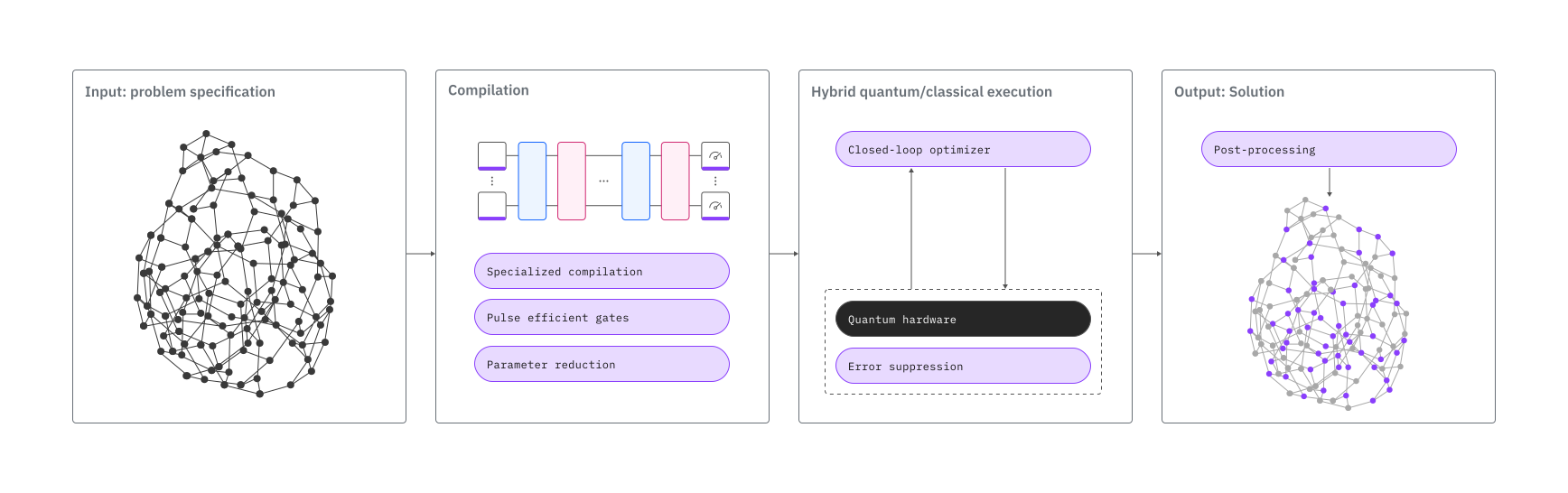
"ソルバーは、ハードウェアレベルでのエラー抑制から、効率的な問題マッピング、クローズドループの古典的最適化まで、アルゴリズム全体を完全に最適化し、自動化します。 その裏では、ソルバーのパイプラインがあらゆる段階でエラーを減らし、有意義なスケーリングに必要なパフォーマンスの向上を可能にしている。 基礎となるワークフローは量子近似最適化アルゴリズム(Quantum Approximate Optimization Algorithm:QAOA)にインスパイアされたもので、これはハイブリッド量子古典アルゴリズムである。 Optimization Solverのワークフローの詳細については、 [発表された原稿を](https://arxiv.org/abs/2406.01743)参照されたい。\n",
"\n",
"\n",
"\n",
"最適化ソルバーで一般的な問題を解く:\n",
"\n",
"1. 問題を目的関数、グラフ、 `SparsePauliOp` スピンチェーンとして定義する。\n",
"2. Qiskitファンクションカタログからファンクションに接続します。\n",
"3. ソルバーで問題を実行し、結果を取得する。\n",
"\n"
]
},
{
"cell_type": "markdown",
"id": "d20af236",
"metadata": {},
"source": [
"\n",
"\n",
"### 対応している問題形式\n",
"\n",
"* 目的関数の多項式表現。 Python、既存の SymPy Polyオブジェクトで作成し、次のようにして文字列に整形するのが理想的です。 [sympy.srepr](https://docs.sympy.org/latest/tutorials/intro-tutorial/printing.html#srepr).\n",
"* 特定の問題タイプのグラフ表現。 グラフは Python の networkx ライブラリを使って作成する。 その後、networkx関数 `[nx.readwrite.json_graph.adjacency_data](http://nx.readwrite.json_graph.adjacency_data.)` を使って文字列に変換する。\n",
"* 特定の問題をスピンの連鎖で表現。 スピンチェインは `SparsePauliOp` オブジェクトとして表現する必要があります。詳細は[ドキュメントを](/docs/api/qiskit/qiskit.quantum_info.SparsePauliOp)参照してください。\n",
"\n",
"\n",
" この関数が現在サポートしていないバックエンドを使用したい場合は、 [Q-CTRLまでご連絡いただき](https://form.typeform.com/to/iuujEAEI?typeform-source=q-ctrl.com)、サポートの追加をご依頼ください。\n",
"\n",
"\n"
]
},
{
"cell_type": "markdown",
"id": "1165f4f0",
"metadata": {},
"source": [
"\n",
"\n",
"## ベンチマーク\n",
"\n",
"[公開されたベンチマーク結果では](https://arxiv.org/abs/2406.01743)、ソルバーが120量子ビット以上の問題を解くことに成功しており、量子アニーリングやトラップドイオンデバイスに関する既発表の結果をも上回っている。 以下のベンチマーク・メトリクスは、いくつかの例に基づいて、問題タイプの精度とスケーリングを大まかに示すものです。 実際の測定基準は、目的関数の項数(密度)やその局所性、変数の数、多項式の次数など、さまざまな問題の特徴によって異なる場合があります。\n",
"\n",
"表示されている \"量子ビット数 \"は難しい制限ではなく、極めて安定した解の精度が期待できる大まかな閾値を表しています。 より大きな問題サイズでも解決に成功しており、この限界を超えたテストが奨励されている。\n",
"\n",
"すべての問題タイプにおいて、任意の量子ビット接続がサポートされている。\n",
"\n",
"| 問題のタイプ | 量子ビット数 | 例 | 正確性 | 合計回数 | ランタイム使用量 (s) | 反復数 |\n",
"| ------------- | ------ | ------------------- | ---- | ---- | ------------ | --- |\n",
"| 疎結合2次問題 | 156 | 3-レギュラー・マックスカット | 100% | 1764 | 293 | 16 |\n",
"| 高次バイナリ最適化 | 156 | イジング・スピングラス模型 | 100% | 1461 | 272 | 16 |\n",
"| 密結合二次問題 | 50 | 完全連結最大カット | 100% | 1758 | 268 | 12 |\n",
"| ペナルティ項を持つ制約問題 | 50 | エッジ密度8%の重み付き最小頂点カバー | 100% | 1074 | 215 | 10 |\n",
"\n"
]
},
{
"cell_type": "markdown",
"id": "73390a19",
"metadata": {},
"source": [
"\n",
"\n",
"## 使用を開始する\n",
"\n",
"まず、 [IBM Quantum](http://quantum.cloud.ibm.com/) のAPIキーを使用して認証を行ってください。 次に、次のようにQiskit関数を選択します。 (このスニペットは[、アカウントが](/docs/guides/functions-get-started#install-qiskit-functions-catalog-client)すでにローカル環境に保存されていることを前提としています。)\n",
"\n"
]
},
{
"cell_type": "code",
"execution_count": 1,
"id": "95a715d2",
"metadata": {},
"outputs": [
{
"data": {
"text/plain": [
"[QiskitFunction(qunova/hivqe-chemistry),\n",
" QiskitFunction(global-data-quantum/quantum-portfolio-optimizer),\n",
" QiskitFunction(algorithmiq/tem),\n",
" QiskitFunction(qedma/qesem),\n",
" QiskitFunction(multiverse/singularity),\n",
" QiskitFunction(ibm/circuit-function),\n",
" QiskitFunction(q-ctrl/optimization-solver),\n",
" QiskitFunction(colibritd/quick-pde),\n",
" QiskitFunction(q-ctrl/performance-management),\n",
" QiskitFunction(kipu-quantum/iskay-quantum-optimizer)]"
]
},
"execution_count": 1,
"metadata": {},
"output_type": "execute_result"
}
],
"source": [
"from qiskit_ibm_catalog import QiskitFunctionsCatalog\n",
"\n",
"catalog = QiskitFunctionsCatalog(channel=\"ibm_quantum_platform\")\n",
"\n",
"# Verify that you have access to the function\n",
"catalog.list()"
]
},
{
"cell_type": "code",
"execution_count": 2,
"id": "8acf84f6",
"metadata": {},
"outputs": [],
"source": [
"# Access Function\n",
"solver = catalog.load(\"q-ctrl/optimization-solver\")"
]
},
{
"cell_type": "markdown",
"id": "e8837f5f",
"metadata": {},
"source": [
"\n",
"\n",
"## 例:制約なし最適化\n",
"\n",
"[最大カット](https://en.wikipedia.org/wiki/Maximum_cut) (max-cut)問題を解く。 以下の例では、156ノードの3正則無重みグラフにおける最大切断問題を用いてソルバーの機能を紹介していますが、重み付きグラフの問題も解くことができます。\n",
"\n"
]
},
{
"cell_type": "markdown",
"id": "a699235b",
"metadata": {},
"source": [
"この例を実行するには、 `qiskit-ibm-catalog` に加え、 `networkx` と `numpy` のパッケージも使用します。 IPythonカーネルを使ってこのサンプルをノートブックで実行している場合は、以下のセルをアンコメントすることでこれらのパッケージをインストールできます。\n",
"\n"
]
},
{
"cell_type": "code",
"execution_count": 3,
"id": "a74fe6a9",
"metadata": {},
"outputs": [],
"source": [
"# %pip install networkx numpy"
]
},
{
"cell_type": "markdown",
"id": "a41c4a0d",
"metadata": {},
"source": [
"\n",
"\n",
"### 1. 問題を定義する\n",
"\n",
"`problem_type='maxcut'`グラフ問題を定義し、を指定することで、最大切断問題を実行できます。\n",
"\n"
]
},
{
"cell_type": "code",
"execution_count": 4,
"id": "d56e1440",
"metadata": {},
"outputs": [],
"source": [
"import networkx as nx\n",
"import numpy as np\n",
"\n",
"# Generate a random graph with 156 nodes\n",
"maxcut_graph = nx.random_regular_graph(d=3, n=156, seed=8)"
]
},
{
"cell_type": "code",
"execution_count": 5,
"id": "0a7255e1",
"metadata": {},
"outputs": [
{
"data": {
"text/plain": [
""
]
},
"metadata": {},
"output_type": "display_data"
}
],
"source": [
"# Optionally, visualize the graph\n",
"nx.draw_networkx(\n",
" maxcut_graph, nx.kamada_kawai_layout(maxcut_graph), node_size=100\n",
")"
]
},
{
"cell_type": "markdown",
"id": "e42a8d55",
"metadata": {},
"source": [
"ソルバーは問題定義の入力として文字列を受け付ける。\n",
"\n"
]
},
{
"cell_type": "code",
"execution_count": 6,
"id": "2546e3e5",
"metadata": {},
"outputs": [],
"source": [
"# Convert graph to string\n",
"problem_as_str = nx.readwrite.json_graph.adjacency_data(maxcut_graph)"
]
},
{
"cell_type": "markdown",
"id": "0ab6f24f",
"metadata": {},
"source": [
"\n",
"\n",
"### 2. 問題を実行する\n",
"\n",
"グラフベースの入力方法を使用する場合は、問題タイプを指定する。\n",
"\n"
]
},
{
"cell_type": "code",
"execution_count": 8,
"id": "16c66d64",
"metadata": {},
"outputs": [],
"source": [
"# Solve the problem\n",
"maxcut_job = solver.run(\n",
" problem=problem_as_str,\n",
" problem_type=\"maxcut\",\n",
" backend_name=backend_name, # E.g. \"ibm_fez\"\n",
")"
]
},
{
"cell_type": "markdown",
"id": "48069093",
"metadata": {},
"source": [
"Qiskit Function [ワーク](/docs/guides/functions-get-started#check-job-status)ロードのステータスを確認したり、 [結果を](/docs/guides/functions-get-started#retrieve-results)返したりするには、次のように操作してください:\n",
"\n"
]
},
{
"cell_type": "code",
"execution_count": 9,
"id": "856fe992",
"metadata": {},
"outputs": [
{
"name": "stdout",
"output_type": "stream",
"text": [
"34b53970-d95a-4e24-8763-fc6f3d112843\n"
]
},
{
"name": "stdout",
"output_type": "stream",
"text": [
"QUEUED\n"
]
}
],
"source": [
"# Print the ID so you can use it later, if necessary\n",
"print(maxcut_job.job_id)\n",
"\n",
"# Get job status\n",
"print(maxcut_job.status())"
]
},
{
"cell_type": "markdown",
"id": "74f48eab",
"metadata": {},
"source": [
"\n",
"\n",
"### 3. 結果を取得する\n",
"\n",
"結果辞書から最適なカット値を取得する。\n",
"\n",
"\n",
" 変数のビット列へのマッピングが変更された可能性があります。 出力辞書にはサブ `variables_to_bitstring_index_map` 辞書が含まれており、順序の検証に役立ちます。\n",
"\n",
"\n"
]
},
{
"cell_type": "code",
"execution_count": 10,
"id": "6b571411",
"metadata": {},
"outputs": [
{
"name": "stdout",
"output_type": "stream",
"text": [
"Optimal cut value: 210.0\n"
]
}
],
"source": [
"# Poll for results\n",
"maxcut_result = maxcut_job.result()\n",
"\n",
"# Take the absolute value of the solution since the cost function is minimized\n",
"qctrl_maxcut = abs(maxcut_result[\"solution_bitstring_cost\"])\n",
"\n",
"# Print the optimal cut value found by the Optimization Solver\n",
"print(f\"Optimal cut value: {qctrl_maxcut}\")"
]
},
{
"cell_type": "markdown",
"id": "508e29b0",
"metadata": {},
"source": [
"のようなオープンソースのソルバーで古典的に問題を解くことで、結果の正確さを検証することができる。 [PuLP](https://coin-or.github.io/pulp/) グラフが密結合でない場合は 高密度の問題では、解を検証するために高度な古典的ソルバーが必要になることがある。\n",
"\n"
]
},
{
"cell_type": "markdown",
"id": "e2817b13",
"metadata": {},
"source": [
"\n",
"\n",
"## 例:制約付き最適化\n",
"\n",
"前述の最大切断問題の例は、一般的な制約なしの二次二値最適化問題である。 Q-CTRLの最適化ソルバーは、制約付き最適化を含む様々な種類の問題に利用できます。 制約条件をペナルティ項としてモデル化した多項式で表される問題定義を入力することで、任意の種類の問題を解くことができます。\n",
"\n",
"次の例は、制約付き最適化問題である[最小頂点カバー](https://en.wikipedia.org/wiki/Vertex_cover) (MVC)のコスト関数を構築する方法を示しています。\n",
"\n"
]
},
{
"cell_type": "markdown",
"id": "a9fbc0e9",
"metadata": {},
"source": [
"`qiskit-ibm-catalog` と `qiskit` パッケージに加え、このサンプルを実行するには以下のパッケージも使用する: `numpy` `networkx`、および `sympy`。 IPythonカーネルを使ってこのサンプルをノートブックで実行している場合は、以下のセルをアンコメントすることでこれらのパッケージをインストールできます。\n",
"\n"
]
},
{
"cell_type": "code",
"execution_count": 11,
"id": "c6428fd0",
"metadata": {},
"outputs": [],
"source": [
"# %pip install numpy networkx sympy"
]
},
{
"cell_type": "markdown",
"id": "98d3bfd3",
"metadata": {},
"source": [
"\n",
"\n",
"### 1. 問題を定義する\n",
"\n",
"ランダムに重み付けされたノードを持つグラフを生成することで、ランダムMVC問題を定義する。\n",
"\n"
]
},
{
"cell_type": "code",
"execution_count": 12,
"id": "c2ce65e3",
"metadata": {},
"outputs": [
{
"data": {
"text/plain": [
""
]
},
"metadata": {},
"output_type": "display_data"
}
],
"source": [
"import networkx as nx\n",
"from sympy import symbols, Poly, srepr\n",
"\n",
"# To change the weights, change the seed to any integer.\n",
"rng_seed = 18\n",
"_rng = np.random.default_rng(rng_seed)\n",
"node_count = 50\n",
"edge_probability = 0.08\n",
"mvc_graph = nx.erdos_renyi_graph(\n",
" node_count, edge_probability, seed=rng_seed, directed=False\n",
")\n",
"\n",
"# add node weights\n",
"for i in mvc_graph.nodes:\n",
" mvc_graph.add_node(i, weight=_rng.random())\n",
"\n",
"# Optionally, visualize the graph\n",
"nx.draw_networkx(mvc_graph, nx.kamada_kawai_layout(mvc_graph), node_size=200)"
]
},
{
"cell_type": "markdown",
"id": "89c91472",
"metadata": {},
"source": [
"重み付けMVCの標準的な最適化モデルは以下のように定式化できる。 まず、エッジが部分集合の頂点に接続されていない場合には、ペナルティを加えなければならない。 したがって、頂点 $i$ がカバーの中にある(つまり部分集合の中にある)場合は $n_i = 1$ とし、そうでない場合は $n_i = 0$ とする。 第二に、目標は部分集合内の頂点の総数を最小化することであり、これは以下の関数で表すことができる:\n",
"\n",
"$\\textbf{Minimize}\\qquad y = \\sum_{i\\in V} \\omega_i n_i$\n",
"\n"
]
},
{
"cell_type": "code",
"execution_count": 13,
"id": "91586ee9",
"metadata": {},
"outputs": [],
"source": [
"# Construct the cost function.\n",
"variables = symbols([f\"n[{i}]\" for i in range(node_count)])\n",
"cost_function = Poly(0, variables)\n",
"\n",
"for i in mvc_graph.nodes():\n",
" weight = mvc_graph.nodes[i].get(\"weight\", 0)\n",
" cost_function += variables[i] * weight"
]
},
{
"cell_type": "markdown",
"id": "9d01684b",
"metadata": {},
"source": [
"さて、グラフのすべての辺は、カバーからの端点を少なくとも1つ含んでいなければならないが、これは不等式で表すことができる:\n",
"\n",
"$n_i + n_j \\ge 1 \\texttt{ for all } (i,j)\\in E$\n",
"\n",
"エッジがカバーの頂点に接続されていない場合は、ペナルティを与えなければならない。 これは、 $P(1-n_i-n_j+n_i n_j)$ ( $P$ は正のペナルティ定数)の形のペナルティを加えることでコスト関数で表すことができる。 従って、重み付きMVCの制約付き不等式に代わる制約なしの不等式は次のようになる:\n",
"\n",
"$\\textbf{Minimize}\\qquad y = \\sum_{i\\in V}\\omega_i n_i + P(\\sum_{(i,j)\\in E}(1 - n_i - n_j + n_i n_j))$\n",
"\n"
]
},
{
"cell_type": "code",
"execution_count": 14,
"id": "1ff1ffcc",
"metadata": {},
"outputs": [],
"source": [
"# Add penalty term.\n",
"penalty_constant = 2\n",
"for i, j in mvc_graph.edges():\n",
" cost_function += penalty_constant * (\n",
" 1 - variables[i] - variables[j] + variables[i] * variables[j]\n",
" )"
]
},
{
"cell_type": "markdown",
"id": "9fd0ba9e",
"metadata": {},
"source": [
"\n",
"\n",
"### 2. 問題を実行する\n",
"\n"
]
},
{
"cell_type": "code",
"execution_count": 15,
"id": "f380b56d",
"metadata": {},
"outputs": [],
"source": [
"# Solve the problem\n",
"mvc_job = solver.run(\n",
" problem=srepr(cost_function),\n",
" backend_name=backend_name, # E.g. \"ibm_fez\"\n",
")"
]
},
{
"cell_type": "markdown",
"id": "d154c226",
"metadata": {},
"source": [
"Qiskit Function [ワーク](/docs/guides/functions-get-started#check-job-status)ロードのステータスを確認したり、 [結果を](/docs/guides/functions-get-started#retrieve-results)返したりするには、次のように操作してください:\n",
"\n"
]
},
{
"cell_type": "code",
"execution_count": 16,
"id": "6de77b14",
"metadata": {},
"outputs": [
{
"name": "stdout",
"output_type": "stream",
"text": [
"QUEUED\n"
]
}
],
"source": [
"print(mvc_job.status())"
]
},
{
"cell_type": "markdown",
"id": "8a95618e",
"metadata": {},
"source": [
"\n",
"\n",
"### 3. 結果を得る\n",
"\n",
"ソリューションを取得し、結果を分析する。 この問題には重み付けノードがあるため、解は単純にカバーされるノードの最小数ではない。 代わりに、解コストは頂点カバーに含まれる頂点の重みの合計を表す。 これは、選択された頂点を使用してグラフ内のすべての辺をカバーするための「コスト」または「重み」の合計を表す。\n",
"\n"
]
},
{
"cell_type": "code",
"execution_count": 17,
"id": "a924bf93",
"metadata": {},
"outputs": [
{
"name": "stdout",
"output_type": "stream",
"text": [
"Solution cost: 10.248198273708624\n"
]
}
],
"source": [
"mvc_result = mvc_job.result()\n",
"qctrl_cost = mvc_result[\"solution_bitstring_cost\"]\n",
"\n",
"# Print results\n",
"print(f\"Solution cost: {qctrl_cost}\")"
]
},
{
"cell_type": "markdown",
"id": "e9ec2e67",
"metadata": {},
"source": [
"\n",
"\n",
"## サポートの利用\n",
"\n",
"ご質問や問題がありましたら、 [Q-CTRLまでご連絡](https://form.typeform.com/to/iuujEAEI?typeform-source=q-ctrl.com)ください。\n",
"\n"
]
},
{
"cell_type": "markdown",
"id": "993aa226c6ec9f5e",
"metadata": {},
"source": [
"\n",
"\n",
"## 変更ログ\n",
"\n",
"* 2026-02-11: 以下のサポートを追加しました `ibm_miami`\n",
"\n"
]
},
{
"cell_type": "markdown",
"id": "5a6a25c8",
"metadata": {},
"source": [
"\n",
"\n",
"## 次のステップ\n",
"\n",
"\n",
" * [Q-CTRL最適化ソルバー](/functions?id=q-ctrl-optimization-solver) へのアクセスをリクエストします。\n",
" * このQiskit関数の [APIリファレンス](/docs/api/functions/q-ctrl-optimization-solver)をご覧ください。\n",
" * [Q-CTRLの最適化ソルバーで高次バイナリ最適化問題を解く](/docs/tutorials/solve-higher-order-binary-optimization-problems-with-q-ctrls-optimization-solver)チュートリアルをお試しください。\n",
" * レビュー [サッチデヴァ, N., et al. (2024). 127量子ビットのゲートモデル量子コンピュータ IBM を用いた量子最適化は、非自明な二値最適化問題において量子アニーリングを超越する性能を発揮し得る。 arXiv プレプリント arXiv:2406.01743](https://arxiv.org/abs/2406.01743).\n",
" * レビュー [・ロコ、D et al. (2026). 量子コンピューターを用いた創薬のための実用的なタンパク質ポケット水和部位予測 arXiv プレプリント arXiv:2512.08390](https://arxiv.org/abs/2512.08390).\n",
" * [マツダの](https://q-ctrl.com/case-study/tackling-a-costly-bottleneck-in-automotive-design)ケーススタディを確認する。\n",
" * [ネットワーク](https://q-ctrl.com/case-study/accelerating-the-schedule-for-quantum-enhanced-rail) ・レールの事例研究を確認する。\n",
" * [オーストラリア](https://q-ctrl.com/case-study/improving-army-logistics-with-quantum-computing)陸軍の事例研究を検討する。\n",
" * [ニューサウスウェールズ州交通局の](https://q-ctrl.com/case-study/delivering-quantum-computing-for-faster-commuting)事例研究を確認する。\n",
"\n",
"\n"
]
},
{
"cell_type": "markdown",
"metadata": {},
"id": "a1b8767d",
"source": "© IBM Corp., 2017-2026"
}
],
"metadata": {
"kernelspec": {
"display_name": "Python 3",
"language": "python",
"name": "python3"
},
"language_info": {
"codemirror_mode": {
"name": "ipython",
"version": 3
},
"file_extension": ".py",
"mimetype": "text/x-python",
"name": "python",
"nbconvert_exporter": "python",
"pygments_lexer": "ipython3",
"version": "3"
}
},
"nbformat": 4,
"nbformat_minor": 5
}