{ "cells": [ { "cell_type": "markdown", "id": "slc-title-0000-4000-8000-000000000000", "metadata": {}, "source": [ "---\n", "title: \"シェーディングされたライトコーンを用いた確率的誤差相殺\"\n", "description: \"シェーディングされたライトコーンを用いた確率的誤差相殺（PEC）を採用し、PECのサンプリングオーバーヘッドを削減するとともに、ハードウェア上での期待値推定における誤差を低減する\"\n", "---\n", "\n", "{/* cspell:ignore samplomatic samplex Trotterized Trotter Lindblad lightcone lightcones Eddins reverser broadcastable postselection postselect antinoise eigval atol starmap unmitigated NoiseLearner PauliLindblad QubitSparsePauli Kingston kicked qubit canonical isa plm qspl Rzz pauli TREX levelname xticks expvals markerfacecolor ncols */}\n", "\n", "\n", "\n", "# シェーディングされたライトコーンを用いた確率的誤差相殺\n", "\n", "*所要時間の目安：Heronプロセッサで10分（注：これはあくまで目安です。（実行時間は状況によって異なる場合があります。）*\n", "\n" ] }, { "cell_type": "markdown", "id": "slc-lout-0000-4000-8000-000000000001", "metadata": {}, "source": [ "\n", "\n", "## 学習成果\n", "\n", "このチュートリアルを学習した後、ユーザーは以下の点を理解できるようになります：\n", "\n", "* 確率的誤差相殺（PEC）とは何か、そしてなぜそのサンプリングオーバーヘッド $\\gamma^2$ が、回路に作用する総ノイズとともに指数関数的に増加するのか\n", "* シェーディングされたライトコーン（SLC）が、各ノイズ項のターゲット観測量への寄与をどのように制限し、重要な部分に緩和リソースを集中できるようにするのか――そして、純粋に幾何学的なライトコーンがすでに提供するバイアスゼロのオーバーヘッド低減に加え、このシェーディングによって、制限された残留バイアスと引き換えに、さらに低いサンプリングオーバーヘッドを実現できる仕組みについて\n", "* とを用いて `NoiseLearnerV3` レイヤーノイズを学習し、と `Executor` プリミティブを通じて `samplomatic` アンチノイズを注入する方法\n", "* ハードウェア上で期待値を推定するために、PECおよびPEC+SLCをTREXおよびポストセレクションと組み合わせる方法\n", "\n", "\n", "\n", "## 前提条件\n", "\n", "このチュートリアルを進める前に、以下のトピックについてあらかじめ理解しておいていただくことをお勧めします：\n", "\n", "* [Qiskit](/docs/guides/intro-to-patterns) のパターンワークフロー\n", "* [Estimatorプリミティブ](/docs/guides/get-started-with-estimator)を用いた観測変数の期待値の計算\n", "* [「推定器プリミティブとエラー軽減オプションの組み合わせ」](/docs/tutorials/combine-error-mitigation-techniques) で取り上げられている、パウリ・トゥワーリングやTREXなどのエラー軽減手法\n", "\n" ] }, { "cell_type": "markdown", "id": "slc-bkgd-0000-4000-8000-000000000002", "metadata": {}, "source": [ "\n", "\n", "## 背景\n", "\n", "このチュートリアルでは、shaded lightcone（SLC）アドオンを使用してエラーを軽減する方法について解説します。このアドオンは、 [確率的誤差相殺（PEC）手法](/docs/guides/error-mitigation-and-suppression-techniques#probabilistic-error-cancellation-pec)を発展させたものであり、ユーザーが回路内の個々の層のノイズを学習し、単一量子ビットゲートや後処理技術を適用することで、そのノイズを相殺するものです。他の手法と比較して、PECはバイアスが軽減された結果に対するより堅牢な境界を提供しますが、QPUの処理時間という点ではオーバーヘッドが大きくなる傾向があります。 PECの実施中、ノイズによる期待値の減衰を補正するために、平均結果は $\\gamma = \\exp(\\sum_{l,\\sigma} 2\\lambda_{l,\\sigma})$ という倍率で再スケーリングされる。ここで、 $\\lambda_{l,\\sigma}$ は、回路の層 $l$ における、学習されたノイズ誤差率（Pauli $\\sigma$ ）である。この再スケーリングにより、分散は $\\gamma^2$ 倍に増加し、その結果、QPU上で必要な回路実行回数も $\\gamma^2$ 倍になる。これを「サンプリングコスト」または「サンプリングオーバーヘッド」と呼ぶ。 $\\gamma$ は指数関数的に増加するため、PECは多くの場合、浅い回路やクビット数の少ない回路に限定される。 [「ノイズの多い量子プロセッサにおける疎なパウリ・リンドブラッドモデルを用いた確率的誤差キャンセル」](https://arxiv.org/abs/2201.09866) で、PECについてさらに詳しく学びましょう。\n", "\n", "軽減する必要のないエラーを特定できれば、このサンプリングコストを指数関数的に削減できる。この方向への第一歩として、局所性を考慮したエラー緩和手法の実装が挙げられる。この手法では、高速に計算可能な従来の「ライトコーン」を用いて、回路全体における観測量の誤差に対する感度を制限することでPECのオーバーヘッドを低減し、一部の問題においてPECの適用範囲をより大規模なものへと拡大する。この光錐の外側にある誤差は、測定結果に影響を及ぼすことはできないため、誤差相殺の手順から除外することができる。この除外により、追加のバイアスを生じさせることなく、サンプリングのオーバーヘッドを、場合によっては大幅に低減することができる。特に、固定深さの回路の局所観測量 $O$ を測定する場合、回路内の量子ビット数を拡大しても、必要なサンプリングオーバーヘッドは最終的に頭打ちとなる（『 [量子回路の局所性とエラー緩和](https://arxiv.org/abs/2303.06496) 』の図 2b を参照）。\n", "\n", "シェーデッド・ライトコーン（SLC）はさらに一歩進んで、古典シミュレーションを用いて、回路全体にわたる誤差に対する感度をより厳密に制限しています。これにより、QPUの処理時間を多少犠牲にしてCPUの処理時間を確保し、バイアスの再正規化に必要なサンプリングのオーバーヘッドを低減します。厳格なカットオフ値を設ける代わりに、回路内の各潜在的な誤差には、その誤差に対する観測量の期待値の影響を受けやすさの上限を示す、段階的な「シェード」が割り当てられる。（後述するバックプロパゲーションによる境界値については、この感受性は回路の初期状態にも依存します。一般的なワークフローや本チュートリアルでは、初期状態はすべてゼロの状態となります。）この精緻な特性解析により、PECをより効率的かつ的を絞って適用し、ばらつきを低減できると同時に、ユーザーは観測可能な推定値におけるバイアスを制御的に調整することが可能となる。詳細については、 [「古典的加速による量子エラー低減のためのライトコーンシェーディング」](https://arxiv.org/abs/2409.04401) を参照してください。\n", "\n", "SLCアドオンのワークフローでは、ライブラ [`samplomatic`](https://qiskit.github.io/samplomatic/guides/index.html) リと、 v0.47.0 で `qiskit-ibm-runtime`Qiskit Runtime に追加されたおよびクラスを活用しており、これにより `Executor``QuantumProgram` 、ユーザーは使いやすさを維持しつつ、エラーの抑制や軽減に関する実行設定をよりモジュール的に制御できるようになります。詳細については、「 [指示型実行モデル](/docs/guides/directed-execution-model)ガイド」をご覧ください。\n", "\n", "\n", "\n", "### SLCエラー軽減ワークフローの概要\n", "\n", "QPUのノイズをモデル化するために、1クビットおよび2クビットのパウリ誤り率を持つ疎なパウリ・リンドブラッドノイズモデルを用い、デバイスの各クビットおよびエッジで局所的に生成されるように設定する。この選択により、本チュートリアルで紹介するSLCエラー軽減ワークフローは以下のようになります：\n", "\n", "a. CPU — 1クビットおよび2クビットのパウリ誤りによる、誤りごとの影響の限界\n", "\n", "1. 前方伝播（観測量に対する境界効果）。各誤差を回路の末端まで伝播させ、観測量とのコミューテータを計算する。\n", " * 計算を扱いやすい範囲に収めるため、進化の過程で演算子の項を切り捨てる。\n", " * 量子速度の限界に基づいて、観測可能量のバックプロパゲーションを緩やかに行うことで、これらの境界をさらに厳密化する。\n", "2. 逆伝播（初期状態に対する境界効果）。各誤差を回路の始点まで伝播させ、初期状態とのコミューテータを計算する。\n", "\n", "b. QPU — ノイズ発生率について学ぶ。を使用して `NoiseLearnerV3` 、パウリ・リンドブラッド雑音モデルの率を推定します。\n", "\n", "c. CPU — 緩和策を優先する\n", "\n", "1. 学習されたノイズ率を用いて、境界を更新する。以前に計算された前方境界と後方境界を組み合わせ、学習されたノイズ率を用いてそれらを更新する。\n", "2. 計算された範囲と学習されたレートを用いて、軽減すべきランクノイズの構成要素をランク付けする。バイアスに与える推定影響度および修正にかかる費用に基づいて、考えられる各ノイズ誤差の優先順位を決定する。\n", "\n", "d. QPU — ノイズ対策機能を挿入して実行する。アノテーションを使用して `Box` 指定したアンチノイズ（逆ノイズ）を適用し、対象の回路を実行します。\n", "\n", "e. CPU — 推定値は観測可能。非マルコフノイズの影響を低減するために、測定に基づく事後選択を適用して、期待値を計算する。\n", "\n", "\n", "\n", "### ノイズ学習の概要\n", "\n", "ノイズ学習は、いくつかの誤差低減手法において一般的な手順であり、 [ノイズ学習器](/docs/guides/noise-learning)によって実行されます。また、 [確率的誤差増幅のチュートリアル](/docs/tutorials/probabilistic-error-amplification)でも取り上げられています。 `NoiseLearnerV3`では、学習対象となるノイズ層をオブジェクトとして [`CircuitInstruction`](/docs/api/qiskit/qiskit.circuit.CircuitInstruction) 具体的に特定できるため、前述の手順に従って各層について所望のSLCノイズ境界を計算することができます。学習済みパウリ・リンドブラッドモデルは、PEC+SLCの優先順位付けに使用される係数を提供します。 `generate_noise_model_paulis`ゲートを層ごとにまとめる方法は、および `find_unique_box_instructions` という `generate_boxing_pass_manager` 便利関数を使用して決定し、その後、以下のステップ2で説明するように、SLCユーティリティ関数に渡しることができます。\n", "\n", "| **パート 1** | **パート 2** | **パート 3** |\n", "| ------------------------------------------------------------------------------------------------------------- | ------------------------------------------------------------------------------------------------------------- | ----------------------------------------------------------------------------------------------------- |\n", "| パウリ・ツイール2量子ビットゲート層 | 層の同一ペアを繰り返し、ノイズを学習する | 忠実度（各ノイズチャネルごとの誤差）を導出する |\n", "| 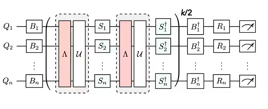![パウリのくるくる回り](https://quantum.cloud.ibm.com/docs/images/tutorials/pec-with-shaded-lightcones/paulitwirl.avif) | ![レイヤーについて学ぶ](https://quantum.cloud.ibm.com/docs/images/tutorials/pec-with-shaded-lightcones/learnlayer.avif) | ![曲線近似](https://quantum.cloud.ibm.com/docs/images/tutorials/pec-with-shaded-lightcones/curvefit.avif) |\n", "\n", "\n", "\n", "### 後処理の概要\n", "\n", "および `Executor` フレーム `samplomatic` ワークを用いて量子ハードウェア上で実行した後、ビットストリングの測定結果を所望の観測量に変換します。このチュートリアルでは、ミラーリングされたアイジング回路（以下のステップ1で構築したもの）を用いたワークフローを解説します。この回路では、回路の後半部分が前半部分の作用を打ち消すため、測定された観測量の理想的な期待値は1となります。関 `executor_expectation_values` 数を用いて観測値を計算する際には、ノイズの影響を低減するためのいくつかの後処理手法を適用しています。これには、非マルコフノイズの影響を受けたショットの除去、読み出し誤差の低減、および当研究におけるPEC実装の詳細への配慮などが含まれる。詳細については、以下のステップ4で説明します。\n", "\n" ] }, { "cell_type": "markdown", "id": "slc-reqs-0000-4000-8000-000000000003", "metadata": {}, "source": [ "\n", "\n", "## 要件\n", "\n", "このチュートリアルを始める前に、以下のものがインストールされていることを確認してください：\n", "\n", "* Qiskit SDK v2.2 またはそれ以降で、 [可視化](/docs/api/qiskit/visualization)機能をサポートしているもの\n", "* Qiskit Runtime v0.47 またはそれ以降 (`pip install qiskit-ibm-runtime`)\n", "* シェーディング付きライトコーン Qiskit アドオン v0.1 以降 (`pip install qiskit-addon-slc`)\n", "* Qiskit アドオン utils v0.3 以降 (`pip install qiskit-addon-utils`)\n", "* Samplomatic v0.13 以降 (`pip install samplomatic`)\n", "\n" ] }, { "cell_type": "markdown", "id": "slc-setup-000-4000-8000-000000000004", "metadata": {}, "source": [ "\n", "\n", "## セットアップ\n", "\n", "まず、このノートブックを実行するために必要なパッケージと関数をインポートします。\n", "\n" ] }, { "cell_type": "code", "execution_count": 1, "id": "946458b7-ab59-448c-8268-f62d8f53bc6d", "metadata": {}, "outputs": [ { "name": "stdout", "output_type": "stream", "text": [ "env: OMP_NUM_THREADS=1\n" ] } ], "source": [ "from multiprocessing import set_start_method\n", "\n", "# Setting this value prevents itertools.starmap deadlock on UNIX systems\n", "set_start_method(\"spawn\")\n", "\n", "# Needed to prevent PySCF from parallelizing internally (SLC only)\n", "%set_env OMP_NUM_THREADS=1" ] }, { "cell_type": "code", "execution_count": 2, "id": "slc-imports-00-4000-8000-000000000005", "metadata": {}, "outputs": [], "source": [ "import numpy as np\n", "from matplotlib import pyplot as plt\n", "\n", "from qiskit import QuantumCircuit\n", "from qiskit.quantum_info import SparsePauliOp\n", "from qiskit.transpiler import generate_preset_pass_manager, PassManager\n", "\n", "from qiskit_ibm_runtime import (\n", " QiskitRuntimeService,\n", " QuantumProgram,\n", " Executor,\n", " NoiseLearnerV3,\n", ")\n", "\n", "import samplomatic\n", "from samplomatic.utils import find_unique_box_instructions\n", "from samplomatic.transpiler import generate_boxing_pass_manager\n", "\n", "from qiskit_addon_utils.exp_vals.measurement_bases import (\n", " get_measurement_bases,\n", ")\n", "from qiskit_addon_utils.exp_vals.expectation_values import (\n", " executor_expectation_values,\n", ")\n", "from qiskit_addon_utils.noise_management import (\n", " gamma_from_noisy_boxes,\n", " trex_factors,\n", ")\n", "from qiskit_addon_utils.noise_management.post_selection import PostSelector\n", "from qiskit_addon_utils.noise_management.post_selection.transpiler.passes import (\n", " AddPostSelectionMeasures,\n", " AddSpectatorMeasures,\n", ")\n", "\n", "from qiskit_addon_slc.bounds import (\n", " compute_backward_bounds,\n", " compute_forward_bounds,\n", " compute_local_scales,\n", " merge_bounds,\n", " tighten_with_speed_limit,\n", ")\n", "from qiskit_addon_slc.utils import (\n", " generate_noise_model_paulis,\n", " map_modifier_ref_to_ref,\n", ")\n", "from qiskit_addon_slc.visualization import draw_shaded_lightcone" ] }, { "cell_type": "markdown", "id": "slc-sim-0000-4000-8000-000000000006", "metadata": {}, "source": [ "\n", "\n", "## 小規模シミュレータの例\n", "\n", "他の学習ベースのエラー低減手法と同様、シェード付きライトコーンを用いたPECは、特定の量子プロセッサに固有の*物理的*ノイズを低減するものであるため、理想的なシミュレータ上には実質的な対応物がないハードウェア機能に依存している：\n", "\n", "* `NoiseLearnerV3` 各固有の2量子ビット層において、スパースなパウリ・リンドブラッドノイズチャネルを実験的に特徴づける。ノイズのないシミュレータでは、除去すべきノイズは存在しない。\n", "* この `Executor` プリミティブは、バックエンド上で `samplomatic` 生成された、ツイール処理が施され、アンチノイズが注入された回路のサンプルを生成します。\n", "\n", "シェーデッド・ライトコーンの境界の計算は古典的な手法ですが、これは学習されたハードウェアノイズ率を基準としてのみ意味を持ちます。このノイズ率が、緩和の許容範囲とサンプリングのオーバーヘッドを決定するからです。こうした理由から、小規模なシミュレータの例は省略し、ハードウェア上で直接PEC+SLCの完全なワークフローを実演します。Qiskitパターンの各ステップについては、以下に詳しく説明します。\n", "\n" ] }, { "cell_type": "markdown", "id": "slc-hw1-0000-4000-8000-000000000007", "metadata": {}, "source": [ "\n", "\n", "## 大規模なハードウェアの例\n", "\n", "IBM Quantum® ハードウェア上で実行される20キュービットのミラーリングされたイジング回路を用いて、Qiskitのパターンに示された4つのステップに従い、PEC+SLCワークフロー全体を実行しました。\n", "\n", "\n", "\n", "### ステップ1：問題の整理\n", "\n", "今回のデモンストレーションは、次のように構成されています：\n", "\n", "1. ここでは、 1D のイジング鎖ハミルトニアンのもとで時間発展を行うことにする。 1D のアイジング鎖は、非常に緻密な回路構造を形成しており、PECの実装例を示すのに適しています。\n", "2. ここでは、観測量 $\\langle X_6 Z_{13}\\rangle$ を測定することにした。この観測量には、 $X$ 成分と $Z$ 成分がそれぞれ1つずつ含まれている。これは、SLCの境界がさまざまな種類のエラーをどのように異なる扱いをするかを強調するのに便利です。\n", "3. この観測量の理想的な期待値が正確に1になるようにしたい。そうすれば、緩和された推定値の質を判断しやすくなるからだ。回路を鏡像反転させれば、ほぼ目的が達成されます。回路の後半にある各ゲートに対して、前半にはその逆のゲートが存在するため、理想的な回路は恒等変換として機能するのです。\n", "4. 最後に、期待値が1という理想的な値を得るためには、回路が観測量の+1の固有状態から開始し――したがって、ミラーリングのおかげで、理想的にはその固有状態で終了することも必要となる。観測可能量は非 $Z$ な成分を含んでおり、プリミティブ `Executor` は回路の終端における所望の測定基底を規定しているため、関 `prepare_basis` 数を用いて、ミラー回路の先頭に、対応する基底準備ゲートを付加する。「」 `get_measurement_bases` 関数を用いて、どのゲートが必要で、どこに配置すべきかを特定するとともに、「標準基底測定」のセクションで論じたように、注釈の規約から `box` 生じる量子ビットインデックスの微妙な点にも注意を払います。\n", "\n" ] }, { "cell_type": "code", "execution_count": 3, "id": "5bfefe99-5958-486e-b8ca-ef2573c7f1e5", "metadata": {}, "outputs": [], "source": [ "# Width of the Ising chain (a free parameter of this demonstration)\n", "num_qubits = 20\n", "\n", "# The observable to measure: one X component (on qubit 6) and one Z component\n", "# (on qubit 13), as motivated in \"Step 1: Map the problem\" above\n", "target_obs_sparse = [(\"XZ\", [6, 13], 1.0)]" ] }, { "cell_type": "code", "execution_count": 4, "id": "e5d4d6d5-9016-4c9a-916b-5075ff459fbf", "metadata": {}, "outputs": [], "source": [ "observable = SparsePauliOp.from_sparse_list(\n", " target_obs_sparse, num_qubits=num_qubits\n", ")" ] }, { "cell_type": "code", "execution_count": 5, "id": "bb40bad8-cb18-4542-9e18-edf5fdfb5452", "metadata": {}, "outputs": [], "source": [ "# Determine the measurement basis each qubit requires for this observable.\n", "# The reverser is used during post-processing in Step 4.\n", "bases_virt, reverser_virt = get_measurement_bases(observable)" ] }, { "cell_type": "code", "execution_count": 6, "id": "5b92fd4e-c559-4c56-8bf6-a6f2e397550c", "metadata": {}, "outputs": [], "source": [ "# Free parameters of the demonstration circuit: the number of Trotter steps\n", "# sets the circuit depth, and rx_angle is the transverse-field rotation angle\n", "# applied in each step (pi/4 makes the dynamics non-Clifford)\n", "num_trotter_steps = 10\n", "rx_angle = np.pi / 4" ] }, { "cell_type": "code", "execution_count": 7, "id": "cc2b001f-c006-45f1-9942-dcbdabefbec4", "metadata": {}, "outputs": [], "source": [ "def construct_ising_circuit(\n", " num_qubits: int,\n", " num_trotter_steps: int,\n", " rx_angle: float,\n", ") -> QuantumCircuit:\n", " circuit = QuantumCircuit(num_qubits)\n", "\n", " for _ in range(num_trotter_steps):\n", " circuit.rx(rx_angle, range(num_qubits))\n", " for first_qubit in (1, 2):\n", " for idx in range(first_qubit, num_qubits, 2):\n", " # equivalent to Rzz(-pi/2):\n", " circuit.sdg([idx - 1, idx])\n", " circuit.cz(idx - 1, idx)\n", "\n", " return circuit\n", "\n", "\n", "def prepare_basis(\n", " circuit: QuantumCircuit, basis: list[int]\n", ") -> QuantumCircuit:\n", " # basis is a list of integer values from 0 to 3. These map to the basis measurement as:\n", " # 0 = I; 1 = Z; 2 = X; 3 = Y\n", " assert len(basis) == circuit.num_qubits\n", "\n", " out_circ = circuit.copy_empty_like()\n", " for qb, bas in enumerate(basis):\n", " if bas == 2:\n", " out_circ.h(qb)\n", " elif bas == 3:\n", " out_circ.rx(-np.pi / 2, qb)\n", "\n", " out_circ.barrier()\n", " out_circ.compose(circuit, inplace=True)\n", " return out_circ\n", "\n", "\n", "def mirror_circuit(circuit: QuantumCircuit) -> QuantumCircuit:\n", " mirror_circ = circuit.copy_empty_like()\n", " mirror_circ.compose(circuit.inverse(), inplace=True)\n", " mirror_circ.barrier()\n", " mirror_circ.compose(circuit, inplace=True)\n", " mirror_circ.measure_active()\n", " return mirror_circ" ] }, { "cell_type": "code", "execution_count": 8, "id": "67553310-f1f0-4736-85ad-bfebd3c00414", "metadata": {}, "outputs": [], "source": [ "# Instantiate the mirrored circuit and prepend the basis-preparation gates\n", "circuit = construct_ising_circuit(num_qubits, num_trotter_steps, rx_angle)\n", "mirrored_circuit = mirror_circuit(circuit)\n", "mirrored_circuit = prepare_basis(mirrored_circuit, bases_virt[0])" ] }, { "cell_type": "code", "execution_count": 9, "id": "0dab284e-dbed-4d2f-92aa-c6c9c0e909a6", "metadata": {}, "outputs": [ { "data": { "text/plain": [ " $\"Output$ " ] }, "execution_count": 9, "metadata": {}, "output_type": "execute_result" } ], "source": [ "mirrored_circuit.draw(\n", " \"mpl\", fold=-1, scale=0.3, idle_wires=False, measure_arrows=False\n", ")" ] }, { "cell_type": "markdown", "id": "slc-step2-000-4000-8000-000000000013", "metadata": {}, "source": [ "\n", "\n", "### ステップ 2：最適化\n", "\n", "実行する回路、測定対象の観測量、およびノイズ学習パラメータに関連する詳細を最適化します。まず、負荷が最も低いHeronプロセッサを選択し、分数ゲートを有効にしてインスタンス化します。これらのフラクショナルゲートにより、当社のポストセレクションフィルタリングの一部において、より高い感度を実現できます。\n", "\n" ] }, { "cell_type": "code", "execution_count": 10, "id": "slc-creds-000-4000-8000-000000000014", "metadata": {}, "outputs": [ { "name": "stdout", "output_type": "stream", "text": [ "Selected backend: ibm_kingston\n" ] } ], "source": [ "# Initialize IBM Quantum Compute Service using your saved credentials\n", "service = QiskitRuntimeService()\n", "\n", "# Select the least busy Heron device. This tutorial targets Heron processors:\n", "# the usage estimate and the non-Markovian-noise post-selection discussed in\n", "# Step 4 are specific to this processor family.\n", "backend = service.least_busy(\n", " operational=True,\n", " simulator=False,\n", " filters=lambda b: b.processor_type[\"family\"] == \"Heron\",\n", ")\n", "# Re-fetch with fractional gates enabled (least_busy does not forward this)\n", "# Fractional gates are enabled so the non-Clifford Rx rotations are supported natively.\n", "backend = service.backend(backend.name, use_fractional_gates=True)\n", "print(f\"Selected backend: {backend.name}\")" ] }, { "cell_type": "markdown", "id": "81dd2580-d4a8-45bb-bd05-707c64aa4ac7", "metadata": {}, "source": [ "まず、 [QPU上で実行するために必要な手順として](/docs/guides/transpile#instruction-set-architecture)、回路をISA命令にトランスパイルします。実行に用いる物理量子ビットの選択は、結果の品質に大きな影響を及ぼします。これは、コヒーレンス時間やゲートの忠実度がデバイスごとに異なり、時間の経過とともに変動するためです。綿密な実験を行う場合、簡単なベンチマーク実験の結果を踏まえてクビットの連鎖を手作業で厳選することは、成果につながる可能性があります（例えば、「 [クビット選択のためのリアルタイム・ベンチマーク](/docs/tutorials/real-time-benchmarking-for-qubit-selection) 」チュートリアルを参照してください）。このチュートリアルの目的上、バックエンドのカップリングマップと最新のキャリブレーションデータに基づいてレイアウトを選択するために、Qiskitトランスパイラーを利用します。\n", "\n" ] }, { "cell_type": "code", "execution_count": 11, "id": "a7505de6-70ef-4996-9f6b-0025f267e920", "metadata": { "scrolled": true }, "outputs": [ { "name": "stdout", "output_type": "stream", "text": [ "Selected layout: [71, 58, 51, 50, 49, 48, 47, 46, 45, 44, 43, 42, 41, 36, 21, 22, 23, 16, 3, 2]\n" ] } ], "source": [ "isa_pm = generate_preset_pass_manager(backend=backend, optimization_level=1)\n", "\n", "isa_circuit = isa_pm.run(mirrored_circuit)\n", "\n", "# The chain of physical qubits selected by the transpiler\n", "layout = isa_circuit.layout.final_index_layout()\n", "print(f\"Selected layout: {layout}\")\n", "\n", "isa_observable = observable.apply_layout(\n", " layout, num_qubits=isa_circuit.num_qubits\n", ")" ] }, { "cell_type": "code", "execution_count": 12, "id": "87f19e08-0cae-4959-9215-354ab099ab02", "metadata": {}, "outputs": [ { "data": { "text/plain": [ " $\"Output$ " ] }, "execution_count": 12, "metadata": {}, "output_type": "execute_result" } ], "source": [ "wire_order = layout + [\n", " q for q in range(isa_circuit.num_qubits) if q not in layout\n", "]\n", "isa_circuit.draw(\n", " \"mpl\",\n", " fold=-1,\n", " scale=0.3,\n", " idle_wires=False,\n", " wire_order=wire_order,\n", " measure_arrows=False,\n", ")" ] }, { "cell_type": "markdown", "id": "7e7135e7-1e86-4d16-b806-30d4a9225e88", "metadata": {}, "source": [ "\n", "\n", "### 回路を枠で囲む\n", "\n", "実装を容易にするため、回路命令を注釈付きボックスに配置するトランスパイレーションパス `generate_boxing_pass_manager` を利用しています。これらのボックスは、PECの場合、回路のどの部分にアンチノイズを注入すべきかを明確に示しています。設定の詳細については、 [Samplomatic](https://qiskit.github.io/samplomatic/) のドキュメントを参照してください。\n", "\n", "なお、SLCワークフローでは、プロセスの後半でを使用 `inject_noise_strategy=\"individual_modification\"` する必要があります。これにより、回路内の命令 `BoxOp` に対する注釈 `InjectNoise` を一意に識別できるようになるためです。（注釈 `InjectNoise` のないボックスは、この方法では特定できません。）\n", "\n", "\n", " SLCバウンド計算では、現在、アノテーションが `InjectNoise` に `site=\"after\"` 配置されていることを前提としています（ [qiskit-addon-slc#33](https://github.com/Qiskit/qiskit-addon-slc/issues/33) を参照）。この設定のデフォルト値は、最近のバージョンで `samplomatic` 変更されたため（ [samplomatic#372](https://github.com/Qiskit/samplomatic/pull/372) を参照）、以下で明示的に設定 `inject_noise_site=\"after\"` します。\n", "\n", "\n", "この `find_unique_box_instructions` 関数は、指定されたボックス化された回路を反復処理し、ノイズ学習およびノイズ注入を目的として、一意の2量子ビット（ 2Q ）層または測定を持つものを特定します。\n", "\n" ] }, { "cell_type": "code", "execution_count": 13, "id": "440f818c-9417-4855-b31b-db47b8595618", "metadata": {}, "outputs": [], "source": [ "# Box circuit with Twirl and InjectNoise annotations\n", "boxes_pm = generate_boxing_pass_manager(\n", " twirling_strategy=\"active\",\n", " inject_noise_strategy=\"individual_modification\",\n", " inject_noise_site=\"after\",\n", " inject_noise_targets=\"gates\",\n", " measure_annotations=\"all\",\n", ")\n", "\n", "\n", "boxed_circuit = boxes_pm.run(isa_circuit)\n", "\n", "# Find the unique instructions (layers) from boxed circuit\n", "unique_2q_instructions = find_unique_box_instructions(\n", " boxed_circuit, normalize_annotations=None, undress_boxes=True\n", ")" ] }, { "cell_type": "code", "execution_count": 14, "id": "d662b076-005e-46c7-826d-4c29a4937404", "metadata": {}, "outputs": [ { "data": { "text/plain": [ " $\"Output$ " ] }, "execution_count": 14, "metadata": {}, "output_type": "execute_result" } ], "source": [ "boxed_circuit.draw(\n", " \"mpl\",\n", " fold=-1,\n", " scale=0.3,\n", " idle_wires=False,\n", " wire_order=wire_order,\n", " measure_arrows=False,\n", ")" ] }, { "cell_type": "markdown", "id": "aa8794ef-7906-4ee3-a9b0-e0399b3e9129", "metadata": {}, "source": [ "\n", "\n", "### 標準塩基の測定の準備\n", "\n", "なお、量子ビットの順序を正確に把握するよう、特に注意を払う必要があります。以下では、回路をボックス化したり一意の命令を特定したりする際にクビットの順序がどのように捉えられるかという点を踏まえ、Executor にクビットの順序を適切に更新して渡す手段として、の `canonical_qubits` 概念について紹介します。詳細については[、Qubitの順序付け規則](https://qiskit.github.io/samplomatic/guides/samplex_io.html#qubit-ordering-convention)に関するドキュメントを参照してください。\n", "\n" ] }, { "cell_type": "code", "execution_count": 15, "id": "e242702b-0274-4ebf-837d-4319a6772339", "metadata": {}, "outputs": [], "source": [ "# Determine the canonical qubits order\n", "meas_box = boxed_circuit.data[-1]\n", "canonical_qubits = [\n", " idx\n", " for idx, qubit in enumerate(boxed_circuit.qubits)\n", " if qubit in meas_box.qubits\n", "]\n", "\n", "# map canonical qubit to physical (isa) qubit\n", "c_2_p = {c: p for c, p in enumerate(canonical_qubits)}\n", "# map physical (isa) qubit to virtual qubit (index in original circuit)\n", "p_2_v = {p: v for v, p in enumerate(layout)}\n", "# compute map between virtual and canonical qubit indices.\n", "c_2_v = {c: p_2_v[p] for c, p in c_2_p.items()}\n", "\n", "assert len(c_2_v) == num_qubits\n", "\n", "bases_canon = [\n", " np.array([base_i[c_2_v[c]] for c in range(num_qubits)], dtype=np.uint8)\n", " for base_i in bases_virt\n", "]" ] }, { "cell_type": "markdown", "id": "61d2762c", "metadata": {}, "source": [ "\n", "\n", "### ライトコーンシェーディング、ノイズ学習、およびアンチノイズ注入のワークフロー\n", "\n", "\n", " このチュートリアルでは、ノイズ学習が完了する前にSLCバウンド計算を実行するため、低減対象の回路は、学習されたノイズモデルに時間的に可能な限り近いタイミングで実行されます。原則として、このワークフローはさらに並列化が可能です。つまり、ノイズ学習ジョブを実行しながら、並行してノイズの境界を推定することができます。任意の量子回路において、ノイズに制約される計算は弱指数関数的な依存性でスケールするため、この制約計算を（例えば、多数のCPUコア間で）並列化することで、与えられた計算時間枠においてより厳しい制約を得ることができ、さらに、QPUによる実行と制約計算自体を並列化することで、最も効率的なワークフローを実現できる。\n", "\n", "\n" ] }, { "cell_type": "markdown", "id": "4a2ec5ed-c339-4273-b407-6bb46b9ede19", "metadata": {}, "source": [ "\n", "\n", "#### 学習予定のノイズモデル「Paulis」を予測する\n", "\n", "ハードウェア上でノイズ学習を実行する前に、まず、ノイズモデルにどのようなパウリ誤差項が含まれるかを列挙する。各層のノイズは、各アクティブ量子ビット上の重み1のパウリ演算（ $X$、 $Y$、または $Z$ ）ごとに1つのエラー率、および接続されたアクティブ量子ビットのペアごとに重み2のパウリ演算ごとに1つのエラー率を持つ疎なパウリ・リンドブラッドモデルとしてモデル化していることを思い出してほしい。この `generate_noise_model_paulis` 関数は、指定された回路の個別のボックス化された各レイヤーを順に処理し、回路の量子ビット間の接続関係を考慮に入れて、まさにこのパウリ項のリストを生成します。\n", "\n", "つまり、このステップでは、後で学習された発生率で埋められることになる `NoiseLearnerV3` ノイズモデルの*構造*を予測するものである。この構造を事前に把握しておくことで、ノイズ学習を実行する前から、発生しうるあらゆる誤差について、上界と下界を計算することが可能になる。\n", "\n" ] }, { "cell_type": "code", "execution_count": 16, "id": "e6783d37-c91f-4c6e-af4e-fb8f37d79e6b", "metadata": {}, "outputs": [], "source": [ "noise_model_paulis = generate_noise_model_paulis(\n", " unique_2q_instructions, backend.coupling_map, boxed_circuit\n", ")" ] }, { "cell_type": "code", "execution_count": 17, "id": "f9fd1389-8c61-4585-85a6-ad17ab7a2f1c", "metadata": {}, "outputs": [], "source": [ "noise_model_rates = {ref: None for ref in noise_model_paulis}" ] }, { "cell_type": "markdown", "id": "942dd468-b2c5-49db-ada5-bcc45024df83", "metadata": {}, "source": [ "\n", "\n", "##### a. 前方境界を計算する\n", "\n", "この `compute_forward_bounds` 関数は、各層のゲートと、前述のように生成されたパウリ項との間の可換関係を、順方向伝播による誤差が目的の観測量 $A$ にどのように影響するかという観点から評価する。パウリ項と可換なゲートについては、何もしない。クリフォードゲートの場合、それらは回路の先頭側に配置されます。クリフォードゲート以外のゲートについては、ターゲット観測量に対するそれらの影響を近似し、後で（すべての上限が統合された後に）ノイズ除去の優先順位付けに活用する。この上界は、まず L2 ノルム（すなわち、関連するパウリ項の係数の二乗和の平方根）を適用することで得られる。関与する量子ビット項が多すぎる場合は、三角不等式を用いたより緩やかな上界に立ち返る。\n", "\n" ] }, { "cell_type": "markdown", "id": "slc-bparam-00-4000-8000-000000000030", "metadata": {}, "source": [ "\n", "\n", "#### 境界計算パラメータを設定する\n", "\n", "以下の設定は、古典的な境界計算を制御します：\n", "\n", "* `slc_atol`: 計算の絶対許容誤差。この閾値を下回る係数を持つ演算子の項は、無視できるものとみなされ、除外されます。\n", "* `slc_eigval_max_qubits`: より厳密な、固有値に基づく（ L2-norm ）上界が評価される量子ビットの最大数。これよりも多くの量子ビットでサポートされる演算については、前述のより緩やかな三角不等式の境界値が適用される。\n", "* `slc_evolution_max_terms`: 回路内で演算子を伝播させる際に保持されるパウリ項の最大数。最小の項を切り捨てることで、境界の精度がわずかに低下する代償を払う代わりに、計算を扱いやすいものに保つことができる。\n", "* `slc_num_processes`: バウンド計算が並列化されるCPUプロセスの数。\n", "* `slc_timeout`: 束縛計算にかかる時間（秒単位）。この予算内で到達できなかったレイヤーには、2 という自明な境界値が割り当てられる。\n", "\n", "\n", " このチュートリアルでは、タイムアウトに達するのは*設計上の意図による*ものです。ノートブックを高速に実行できるように、またタイムアウトに達しても安全であることを示すために、意図的にタイムアウト時間を短く設定 `slc_timeout` しています。計算されたシェードは各段階における上限値であるため、タイムアウトが発生しても、到達しなかったレイヤーについてはその上限値が（自明な値へと）緩くなるだけであり、エラーの影響を過小評価することは決してありません。これは、以下の可視化図において、左端のレイヤーがすべて自明な境界で塗りつぶされている様子として表れています。タイムアウトを長くする（またはプロセス数を増やす）ことで、範囲が狭まり、サンプリングのオーバーヘッドがさらに軽減されます。\n", "\n", "\n" ] }, { "cell_type": "code", "execution_count": 18, "id": "79fe4a21-b80d-496b-ba20-f16d9b11834d", "metadata": {}, "outputs": [], "source": [ "slc_atol = 1e-8\n", "slc_eigval_max_qubits = 18\n", "slc_evolution_max_terms = 1000\n", "slc_num_processes = 8\n", "slc_timeout = 60" ] }, { "cell_type": "code", "execution_count": 19, "id": "705fcb9f-c753-45a6-97dd-9ff8ecb07018", "metadata": { "scrolled": true }, "outputs": [ { "name": "stderr", "output_type": "stream", "text": [ "Bounds computation timed out.\n" ] } ], "source": [ "forward_bounds = compute_forward_bounds(\n", " boxed_circuit,\n", " noise_model_paulis,\n", " isa_observable,\n", " evolution_max_terms=slc_evolution_max_terms,\n", " eigval_max_qubits=slc_eigval_max_qubits,\n", " atol=slc_atol,\n", " num_processes=slc_num_processes,\n", " timeout=slc_timeout,\n", ")" ] }, { "cell_type": "markdown", "id": "aaf7c188-c85b-42cf-a096-0a5dc72a68e3", "metadata": {}, "source": [ "\n", "\n", "#### 手作業による検査のためにSLCを可視化する\n", "\n", "陰影で示された境界の挙動については、測定項とパウリ項が局所誤差とどのように相互作用するかを検討することで解釈することができます。これらのパターンは、このキック付きアイジング・ハミルトニアンによる時間発展問題に特徴的なものであり、論文『 [Lightcone Shading for Classically Accelerated Quantum Error Mitigation](https://arxiv.org/abs/2409.04401)』にも見られ、いくつかの顕著な特徴を備えている：\n", "\n", "* 観測量に含まれる2つの非自明なパウリ演算から生じる2つのコーンを、はっきりと区別することができる。\n", "* キュービット6に対するX測定は、最右層のXエラーと可換であることがわかる。\n", "* キュービット13のZパウリ演算が、右端の層にあるZエラーと可換であることがわかります。\n", "* 上記で指定されたタイムアウトに達すると、左側の残りの層はすべて、値が2の単純な境界で埋め尽くされます。\n", "\n" ] }, { "cell_type": "code", "execution_count": 20, "id": "285edaef-8e79-41eb-a563-4675ea75d5b1", "metadata": {}, "outputs": [ { "data": { "text/plain": [ " $\"Output$ " ] }, "metadata": {}, "output_type": "display_data" }, { "data": { "text/plain": [ " $\"Output$ " ] }, "metadata": {}, "output_type": "display_data" }, { "data": { "text/plain": [ " $\"Output$ " ] }, "metadata": {}, "output_type": "display_data" } ], "source": [ "for p in \"XYZ\":\n", " display(\n", " draw_shaded_lightcone(\n", " boxed_circuit,\n", " forward_bounds,\n", " noise_model_paulis,\n", " pauli_filter=p,\n", " scale=0.15,\n", " fold=-1,\n", " idle_wires=False,\n", " wire_order=wire_order,\n", " measure_arrows=False,\n", " )\n", " )" ] }, { "cell_type": "markdown", "id": "1aee6b29-8077-4019-9e37-3e80292aadf6", "metadata": {}, "source": [ "\n", "\n", "#### b. 量子速度の限界を用いて前方境界を厳密化する\n", "\n", "次に、関数を `tighten_with_speed_limit` 用いて、その境界をさらに厳密にします。観測対象の光錐の幾何学的広がりは、上記で計算された前方境界においてすでに完全に考慮されている。この関数が追加するのは、回路内を情報が流れる速度の制限（2量子ビットゲートの層ごとに、ライトコーンは最大で1量子ビットずつしか拡大しない）を活用した自己一貫性チェックであり、これにより、以前に計算された各境界値間の関係をさらに厳密に調整する。情報は双方向に流れています：\n", "\n", "1. コミューテーターの境界から、バックプロパゲーションされた観測量の境界について：ある観測量がクビット上の $Z$ 誤差と可換である場合、その観測量には、 $X$ や $Y$ の成分がほとんど含まれていないことになる。\n", "2. バックプロパゲーションされた観測量の境界から、コミューテーターの境界について：ある量子ビットにおいて、その観測量の $X$ および $Y$ 成分がごくわずかであるならば、その量子ビットにおける $Z$ とはほぼ可換でなければならない。\n", "\n" ] }, { "cell_type": "code", "execution_count": 21, "id": "e060d547-79da-4f54-bf5e-677f70306040", "metadata": { "scrolled": true }, "outputs": [], "source": [ "forward_bounds_tighter = tighten_with_speed_limit(\n", " forward_bounds, boxed_circuit, noise_model_paulis, isa_observable\n", ")" ] }, { "cell_type": "markdown", "id": "85f3c9c2-d60c-4044-a496-dae88c3dd749", "metadata": {}, "source": [ "\n", "\n", "#### 手作業による検査のためにSLCを可視化する\n", "\n", "原則として、この厳格化により、計算された境界と、タイムアウトを超えたレイヤーに割り当てられた自明な境界との間の移行がよりスムーズになります。この例では、タイムアウトに達する頃には光錐がすでに回路の端まで広がってしまっているため、その影響はほとんど目に見えません。\n", "\n" ] }, { "cell_type": "code", "execution_count": 22, "id": "6ba4b397-e903-4b85-9482-31a96c689dc0", "metadata": {}, "outputs": [ { "data": { "text/plain": [ " $\"Output$ " ] }, "metadata": {}, "output_type": "display_data" }, { "data": { "text/plain": [ " $\"Output$ " ] }, "metadata": {}, "output_type": "display_data" }, { "data": { "text/plain": [ " $\"Output$ " ] }, "metadata": {}, "output_type": "display_data" } ], "source": [ "for p in \"XYZ\":\n", " display(\n", " draw_shaded_lightcone(\n", " boxed_circuit,\n", " forward_bounds_tighter,\n", " noise_model_paulis,\n", " pauli_filter=p,\n", " scale=0.15,\n", " fold=-1,\n", " idle_wires=False,\n", " wire_order=wire_order,\n", " measure_arrows=False,\n", " )\n", " )" ] }, { "cell_type": "markdown", "id": "ce0f9cf4-565a-4f18-baa5-bec5c7b354a2", "metadata": {}, "source": [ "\n", "\n", "#### c. 後方境界を計算する\n", "\n", "ノイズ予測のこの部分では、特定の層における誤差が、入力状態 $\\rho$ にどのような影響を与えるかを評価する。この `compute_backward_bounds` 関数は、まず回路を反転させて測定ゲートを除去し、その後、順方向計算の場合と同様の解析を行う。\n", "\n" ] }, { "cell_type": "code", "execution_count": 23, "id": "ff895191-feda-4958-a58a-3d1fb973cb68", "metadata": { "scrolled": true }, "outputs": [], "source": [ "backward_bounds = compute_backward_bounds(\n", " boxed_circuit,\n", " noise_model_paulis,\n", " evolution_max_terms=slc_evolution_max_terms,\n", " num_processes=slc_num_processes,\n", " timeout=slc_timeout,\n", ")" ] }, { "cell_type": "markdown", "id": "c707d352-37fe-4c53-82a3-a1207b7a7bfc", "metadata": {}, "source": [ "\n", "\n", "#### 手作業による検査のためにSLCを可視化する\n", "\n", "後方境界を計算することで、初期状態の構造が誤差伝播の初期段階の挙動をどのように左右しているかがわかります：\n", "\n", "* Z誤差が、初期状態 |0⟩ と当初どのように可換であるかがはっきりと見て取れる。\n", "* X基底の+1固有状態を初期化する量子ビット6においてのみ、Zエラーは可換性を満たさないのに対し、Xエラーは可換性を満たす。\n", "\n" ] }, { "cell_type": "code", "execution_count": 24, "id": "40d0eba9-5e0b-4b1d-8fb2-c239e262062f", "metadata": {}, "outputs": [ { "data": { "text/plain": [ " $\"Output$ " ] }, "metadata": {}, "output_type": "display_data" }, { "data": { "text/plain": [ " $\"Output$ " ] }, "metadata": {}, "output_type": "display_data" }, { "data": { "text/plain": [ " $\"Output$ " ] }, "metadata": {}, "output_type": "display_data" } ], "source": [ "for p in \"XYZ\":\n", " display(\n", " draw_shaded_lightcone(\n", " boxed_circuit,\n", " backward_bounds,\n", " noise_model_paulis,\n", " pauli_filter=p,\n", " scale=0.15,\n", " fold=-1,\n", " idle_wires=False,\n", " wire_order=wire_order,\n", " measure_arrows=False,\n", " )\n", " )" ] }, { "cell_type": "markdown", "id": "c8960e51-733e-4458-b77c-287ba3abdb8d", "metadata": {}, "source": [ "\n", "\n", "#### 学習されたノイズ率を使用せずに、統合された境界をプレビューする\n", "\n", "この `merged_bounds` 関数は、回路内のどの点で、逆方向の境界から順方向の境界への切り替えを行うと、目的の観測量に対する推定バイアスの総和が最小になるかを決定する。このバイアスは、その点より前のすべてのノイズ位置に対する後方方向の寄与の合計に、その点より後のすべてのノイズ位置に対する前方方向の寄与を加えたものとして計算される。現在、これはすべての量子ビットに対して一律に行われています。\n", "\n", "\n", " 後方境界から前方境界に切り替える最適な時点は、学習されたノイズ率によって決まる。現段階では、発生率はまだ設定されていません。 `noise_model_rates` 各層について、はに `None` 初期化されており、これは `merge_bounds` 一様なノイズ発生率として扱われます。したがって、ここに示されている統合された境界はあくまでプレビューに過ぎません。ステップ3では、実際に学習されたレートを用いてこれらを再計算します。\n", "\n", "\n" ] }, { "cell_type": "code", "execution_count": 25, "id": "b5cd8752-3bb5-44ee-97a8-6edaf5946e9d", "metadata": {}, "outputs": [ { "name": "stderr", "output_type": "stream", "text": [ "Missing noise rates. Partitioning backward/forward commutator bounds by assuming uniform error rates.\n", "Optimal spacetime partitioning not implemented!Just partitioning list of noisy boxes.\n" ] } ], "source": [ "merged_bounds = merge_bounds(\n", " boxed_circuit,\n", " forward_bounds_tighter,\n", " backward_bounds,\n", " noise_model_rates,\n", ")" ] }, { "cell_type": "markdown", "id": "ace27801-b949-44e0-801d-e74ccb2f877a", "metadata": {}, "source": [ "\n", "\n", "### 手作業による検査のためにSLCを可視化する\n", "\n", "後方境界と引き締められた前方境界を統合すると、統合されたSLCの挙動が明らかになります：\n", "\n", "* 上記の関数は、後方境界から引き締められた前方境界への切り替えが行われるパーティションが選択されることを示しています。\n", "* 以下からわかるように、SLCには現在、部分的な後方境界と部分的な引き締められた前方境界が含まれている。\n", "\n" ] }, { "cell_type": "code", "execution_count": 26, "id": "eb2948bc-fa27-4108-b03c-0291d3b2f7c8", "metadata": {}, "outputs": [ { "data": { "text/plain": [ " $\"Output$ " ] }, "metadata": {}, "output_type": "display_data" }, { "data": { "text/plain": [ " $\"Output$ " ] }, "metadata": {}, "output_type": "display_data" }, { "data": { "text/plain": [ " $\"Output$ " ] }, "metadata": {}, "output_type": "display_data" } ], "source": [ "for p in \"XYZ\":\n", " display(\n", " draw_shaded_lightcone(\n", " boxed_circuit,\n", " merged_bounds,\n", " noise_model_paulis,\n", " pauli_filter=p,\n", " scale=0.15,\n", " fold=-1,\n", " idle_wires=False,\n", " wire_order=wire_order,\n", " measure_arrows=False,\n", " )\n", " )" ] }, { "cell_type": "markdown", "id": "slc-step3-000-4000-8000-000000000050", "metadata": {}, "source": [ "\n", "\n", "### ステップ3：実行\n", "\n", "このセクションでは、実際の量子デバイスを使用するワークフローの段階に入ります。この学習ベースのエラー軽減手法には、2つのステップがあります：\n", "\n", "1. `NoiseLearnerV3`を使用して、その音を覚えてください。\n", "2. および `Executor` フレームワーク `samplomatic` を用いて、エラー軽減回路を実行する。\n", "\n", "量子回路から得られる誤差の上限値をもとに、関連するノイズ率を把握し、エラーバジェットの優先順位付けを行い、サンプリングのオーバーヘッドを決定した上で、QPU上で実行します。\n", "\n" ] }, { "cell_type": "markdown", "id": "slc-nlmd-0000-4000-8000-000000000051", "metadata": {}, "source": [ "\n", "\n", "### a. 騒音基準値を学ぶ\n", "\n", "ノイズ学習器は、スパース[なパウリ・リンドブラッドノイズモデル](https://arxiv.org/abs/2201.09866)に基づき、対象となる1つ以上の回路内のゲートに影響を与えるノイズ過程を特徴付けます。この `run()` メソッドは、noise-learnerの設定で指定されたオプションを使用して、指定された一意の2量子ビット層に対してノイズ学習ジョブを起動します。これらのオプションは、パウリ・トゥイール戦略、ランダム化とショットの回数、学習深度、およびポストセレクションを制御します。\n", "\n", "また、学習の深さも意図的に選定しています。学習ベースの緩和策に関する実用的な知見として、 `samplomatic` 緩和対象とする回路の深さと、学習の最大深さを一致させることが極めて有益であることが挙げられる。 NLv3`layer_pair_depths`\\* は\\*レイヤーペア（レイヤーとその逆）単位で測定されるため、最深値は回路の2量子ビットレイヤーの深さの半分に設定します。\n", "\n" ] }, { "cell_type": "code", "execution_count": 27, "id": "slc-psflag-00-4000-8000-000000000052", "metadata": {}, "outputs": [], "source": [ "post_selection_enabled = True" ] }, { "cell_type": "code", "execution_count": 28, "id": "slc-nlopt-00-4000-8000-000000000053", "metadata": {}, "outputs": [], "source": [ "# Match the deepest noise-learning depth to the depth of the circuit being\n", "# mitigated. NLv3 ``layer_pair_depths`` are measured in layer pairs (a layer\n", "# plus its inverse), so the deepest value is half the circuit's two-qubit-layer\n", "# depth. Learning to this depth markedly improves the quality of the mitigation.\n", "#\n", "# We measure the two-qubit-layer depth on the pre-boxed ISA circuit: after\n", "# boxing, every two-qubit gate is hidden inside a full-width ``BoxOp``, so a\n", "# ``num_qubits == 2`` filter on ``boxed_circuit`` matches nothing (and\n", "# ``QuantumCircuit.depth`` does not recurse into boxes).\n", "depth_2q = isa_circuit.depth(lambda instr: instr.operation.num_qubits == 2)\n", "max_layer_pair_depth = depth_2q // 2 # dividing by 2 since we want pairs\n", "\n", "# Use a fixed schedule of learning depths, but drop any that exceed the circuit's\n", "# depth and always cap the deepest value at ``max_layer_pair_depth`` so we never\n", "# learn deeper than the circuit being mitigated.\n", "candidate_depths = [1, 2, 4, 8, 12, 16, 24, 32, 40, 48]\n", "layer_pair_depths = sorted(\n", " {d for d in candidate_depths if d < max_layer_pair_depth}\n", " | {max_layer_pair_depth}\n", ")\n", "\n", "noise_learner_options = {\n", " \"num_randomizations\": 64,\n", " \"shots_per_randomization\": 128,\n", " \"layer_pair_depths\": layer_pair_depths,\n", " \"post_selection\": {\n", " \"enable\": post_selection_enabled,\n", " \"strategy\": \"edge\",\n", " \"x_pulse_type\": \"rx\",\n", " },\n", " \"environment\": {\"job_tags\": [\"TUT_SLC\"]},\n", "}\n", "\n", "noise_learner = NoiseLearnerV3(backend, noise_learner_options)" ] }, { "cell_type": "code", "execution_count": 29, "id": "slc-nlrun-00-4000-8000-000000000054", "metadata": {}, "outputs": [], "source": [ "noise_learner_job = noise_learner.run(unique_2q_instructions)" ] }, { "cell_type": "code", "execution_count": 30, "id": "db624045-7abe-41f1-a60c-1ba141aaa6f6", "metadata": {}, "outputs": [], "source": [ "noise_learner_result = noise_learner_job.result()" ] }, { "cell_type": "code", "execution_count": 31, "id": "b08c37a6-5acb-41e9-a76c-abc0195d87f7", "metadata": {}, "outputs": [ { "name": "stdout", "output_type": "stream", "text": [ "Minimum fraction of shots kept for noise learning experiments: 0.71\n" ] } ], "source": [ "if post_selection_enabled:\n", " print(\n", " \"Minimum fraction of shots kept for noise learning experiments: \",\n", " end=\"\",\n", " )\n", " print(\n", " f\"{min([min(d.values()) for d in [nlr.metadata['post_selection']['fraction_kept'] for nlr in noise_learner_result[:2]]]):.2f}\"\n", " )" ] }, { "cell_type": "code", "execution_count": 32, "id": "99144d7f-b891-4115-8cb3-ecdbedd10a73", "metadata": {}, "outputs": [], "source": [ "# Get a dict mapping each InjectNoise.ref to its learned PauliLindbladMap\n", "refs_2_plm = noise_learner_result.to_dict(\n", " unique_2q_instructions, require_refs=False\n", ")" ] }, { "cell_type": "markdown", "id": "e6a790a3-bc11-46e2-8cb4-2e43257926c8", "metadata": {}, "source": [ "\n", "\n", "### b.i. 学習された実際のノイズ率に基づいて、境界を更新する\n", "\n", "特定のノイズモデルが学習されたことで、学習されたノイズ率を予測されたノイズの範囲に適用し、バイアスを最小化する上でどの範囲が最も大きな影響を与えるかを最終的に特定することができる。\n", "\n" ] }, { "cell_type": "code", "execution_count": 33, "id": "bba8fca6-5339-4d4d-be01-45ca8bf94a5a", "metadata": {}, "outputs": [ { "name": "stderr", "output_type": "stream", "text": [ "Optimal spacetime partitioning not implemented!Just partitioning list of noisy boxes.\n" ] } ], "source": [ "merged_bounds = merge_bounds(\n", " boxed_circuit,\n", " forward_bounds_tighter,\n", " backward_bounds,\n", " refs_2_plm,\n", ")" ] }, { "cell_type": "markdown", "id": "649b9640-e89f-4021-9f7d-f1e136c4eb6d", "metadata": {}, "source": [ "\n", "\n", "#### b.ii. ハードウェア実行におけるを `local_scales` 計算する\n", "\n", "`compute_local_scales` 回路内で起こりうる各ノイズ誤差を検討し、その誤差が最終的な測定値にどの程度のバイアスを及ぼすか、またそれを補正するのにどれほどのコストがかかるかを推定する。その後、エラーを「軽減する価値」が高い順にランク付けし、許容されるサンプリングコストの範囲内（あるいは所望の精度を達成しつつ）で、バイアスを可能な限り低減できるサブセットを選択する。その結果、どの誤差が積極的に軽減され、どの誤差が軽減されないかを示す一連のスケーリング係数（`local_scales`）に加え、予測される総サンプリングコストのオーバーヘッド（`sampling_costs`）および残存バイアス（`residual_bias_bound`）が得られる。\n", "\n", "所望の残留バイアスを制御できることは、PECのSLC実装における重要な特徴である。 [元の実装](https://arxiv.org/abs/2201.09866)では、サンプリングのオーバーヘッドは常にバイアスをゼロにすることを目指していましたが、期待される残存バイアスとのトレードオフによって、必要なサンプリングのオーバーヘッドを調整することができます。これにより、ユーザーは所定のサンプリング予算の範囲内に収めることができます。これは、ワークフローの初期段階でのプロトタイプ作成において特に役立ちます。\n", "\n" ] }, { "cell_type": "code", "execution_count": 34, "id": "8914e00e-ba21-41dc-9e64-b942bb23fde1", "metadata": {}, "outputs": [], "source": [ "id_map = map_modifier_ref_to_ref(boxed_circuit)" ] }, { "cell_type": "code", "execution_count": 35, "id": "4c971d31-f2b4-4d17-8a83-4f6d14f81f6f", "metadata": { "scrolled": true }, "outputs": [ { "name": "stdout", "output_type": "stream", "text": [ "Full PEC gamma=12.750876317157042, sampling cost (gamma^2) = 162.58484685543633\n" ] } ], "source": [ "summed_rates = 0.0\n", "for box_id, noise_id in id_map.items():\n", " learned_plm = refs_2_plm[noise_id]\n", " summed_rates += np.sum(learned_plm.rates)\n", " # print(f\"{box_id}:\\tgamma = {np.exp(2 * summed_rates):1.6e}\\tsampling cost = {np.exp(4 * summed_rates):1.6e}\")\n", "total_gamma = np.exp(2 * summed_rates)\n", "print(\n", " f\"Full PEC gamma={total_gamma}, sampling cost (gamma^2) = {total_gamma**2}\"\n", ")" ] }, { "cell_type": "code", "execution_count": 36, "id": "fb6f2aa0-8a35-420c-aae3-6fc5e9aa8747", "metadata": {}, "outputs": [], "source": [ "biases = []\n", "costs = []\n", "for bias in [0.0] + np.arange(0.001, 0.102, 0.01).tolist():\n", " _, cost_, bias_ = compute_local_scales(\n", " boxed_circuit,\n", " merged_bounds,\n", " refs_2_plm,\n", " sampling_cost_budget=np.inf,\n", " bias_tolerance=bias,\n", " )\n", " biases.append(bias_)\n", " costs.append(cost_)" ] }, { "cell_type": "markdown", "id": "slc-trade-00-4000-8000-000000000065", "metadata": {}, "source": [ "\n", "\n", "#### サンプリングのオーバーヘッドと残留バイアスのバランスをとる\n", "\n" ] }, { "cell_type": "code", "execution_count": 37, "id": "slc-ovplot-0-4000-8000-000000000066", "metadata": {}, "outputs": [ { "data": { "text/plain": [ "Text(0.5, 0.98, 'PEC sampling overhead reduction due to SLC')" ] }, "execution_count": 37, "metadata": {}, "output_type": "execute_result" }, { "data": { "text/plain": [ " $\"Output$ " ] }, "metadata": {}, "output_type": "display_data" } ], "source": [ "xticks = np.arange(0, 11)\n", "\n", "fig, ax = plt.subplots()\n", "ax.scatter(\n", " [0], [total_gamma**2], marker=\"D\", c=\"tab:orange\", label=\"full PEC\"\n", ")\n", "ax.plot(\n", " 100 * np.array(biases),\n", " np.array(costs),\n", " \"o-\",\n", " c=\"tab:blue\",\n", " label=\"PEC+SLC\",\n", ")\n", "ax.set_yscale(\"log\")\n", "ax.set_xticks(xticks, [f\"{x:.1f}\" for x in xticks])\n", "\n", "ax.set_xlabel(\"Remaining bias [%]\")\n", "ax.set_ylabel(r\"Sampling overhead, $\\gamma^2$\")\n", "ax.grid()\n", "ax.legend()\n", "fig.suptitle(\"PEC sampling overhead reduction due to SLC\")" ] }, { "cell_type": "code", "execution_count": 38, "id": "1df482f9-c12c-4ea7-a71e-7ffc0837b5a6", "metadata": {}, "outputs": [], "source": [ "chosen_bias_thres = 0.1" ] }, { "cell_type": "code", "execution_count": 39, "id": "slc-lscale-0-4000-8000-000000000068", "metadata": {}, "outputs": [ { "name": "stdout", "output_type": "stream", "text": [ "PEC+SLC sampling cost (gamma^2) = 48.13646509622307 w/ remaining bias = 10.0%\n" ] } ], "source": [ "local_scales, sampling_cost, residual_bias_bound = compute_local_scales(\n", " boxed_circuit,\n", " merged_bounds,\n", " refs_2_plm,\n", " sampling_cost_budget=np.inf,\n", " bias_tolerance=chosen_bias_thres,\n", ")\n", "print(\n", " f\"PEC+SLC sampling cost (gamma^2) = {sampling_cost} \"\n", " f\"w/ remaining bias = {100 * residual_bias_bound:.1f}%\"\n", ")" ] }, { "cell_type": "markdown", "id": "8b03c0ed-d026-4b29-bc09-68c4d0c94889", "metadata": {}, "source": [ "\n", "\n", "### c. antinoise を使用して、対象の回路を実行する\n", "\n", "\n", "\n", "#### c.i. 以下の方法を使用して、テンプレート回路を準備します。 `samplex`\n", "\n", "`template_circuit`これは `samplex` 、Samplomaticのメソッド `build` の出力であり、のランダム化されたパラメータを生成するために必要なすべての情報がエンコードされています。これらは、オブジェクト `QuantumProgram` の設定に使用され、そのオブジェクトは、プリミティブ `Executor` とともにQPU上で実行されます。 `samplex`それぞれ `QuantumProgram` には複数の項目を含めることができ、これらはとの `template` ペアとして考えることができます。\n", "\n", "詳細については[、「Hello samplomatic](https://github.com/qiskit-community/qdc-challenges-2025/blob/main/day3_tutorials/Track_A/hello_samplomatic/Samplomatic%20-%20Hello%20World.ipynb) 」のチュートリアルをご覧ください。\n", "\n" ] }, { "cell_type": "code", "execution_count": 40, "id": "a68109cc-3b38-40e0-b145-edaa06b9934d", "metadata": {}, "outputs": [], "source": [ "# Build template circuit and samplex for later use with the \"Executor\"\n", "template_circuit, samplex = samplomatic.build(boxed_circuit)" ] }, { "cell_type": "code", "execution_count": 41, "id": "0de4922b-b958-48d7-b63a-819edfb354bd", "metadata": {}, "outputs": [], "source": [ "# Set up postselection if it's been enabled\n", "if post_selection_enabled:\n", " # Set up post selection PM (to add PS instructions)\n", " post_selection_pm = PassManager(\n", " [\n", " AddSpectatorMeasures(backend.coupling_map),\n", " AddPostSelectionMeasures(x_pulse_type=\"rx\"),\n", " ]\n", " )\n", " final_template_circuit = post_selection_pm.run(template_circuit)\n", "else:\n", " final_template_circuit = template_circuit" ] }, { "cell_type": "markdown", "id": "4f00c61a-4c4d-40d9-9a41-11ea8e9a9337", "metadata": {}, "source": [ "\n", "\n", "#### c.ii. を設定する `QuantumProgram`\n", "\n" ] }, { "cell_type": "code", "execution_count": 42, "id": "a63d8881-2bbb-4c99-afd3-43f03ee04e5c", "metadata": {}, "outputs": [], "source": [ "num_randomizations = 4096\n", "shots_per_randomization = 64\n", "chunk_size = 256" ] }, { "cell_type": "code", "execution_count": 43, "id": "038a04c9-20ba-432c-bfec-cf69e67ac82f", "metadata": {}, "outputs": [], "source": [ "# Set up QuantumProgram\n", "program = QuantumProgram(shots=shots_per_randomization, noise_maps=refs_2_plm)\n", "\n", "# no EM\n", "\n", "# Collect up a dict of the other arguments that need to be bound to samplex_inputs\n", "samplex_inputs = {\n", " f\"noise_scales.{ref}\": float(0) for ref in local_scales.keys()\n", "}\n", "samplex_inputs |= {\"basis_changes\": {\"basis0\": bases_canon[0]}}\n", "\n", "# Convert samplex_inputs into a dict to pass to QuantumProgram\n", "samplex_arguments = (\n", " samplex.inputs().bind(**samplex_inputs).make_broadcastable()\n", ")\n", "\n", "program.append_samplex_item(\n", " circuit=final_template_circuit,\n", " samplex=samplex,\n", " samplex_arguments=samplex_arguments,\n", " shape=(num_randomizations,),\n", " chunk_size=chunk_size,\n", ")\n", "\n", "# plain PEC\n", "\n", "# Collect a dict of the other arguments that need to be bound to samplex_inputs\n", "samplex_inputs = {\n", " f\"noise_scales.{ref}\": float(-1) for ref in local_scales.keys()\n", "}\n", "samplex_inputs |= {\"basis_changes\": {\"basis0\": bases_canon[0]}}\n", "\n", "# Convert samplex_inputs into a dict to pass to QuantumProgram\n", "samplex_arguments = (\n", " samplex.inputs().bind(**samplex_inputs).make_broadcastable()\n", ")\n", "\n", "program.append_samplex_item(\n", " circuit=final_template_circuit,\n", " samplex=samplex,\n", " samplex_arguments=samplex_arguments,\n", " shape=(num_randomizations,),\n", " chunk_size=chunk_size,\n", ")\n", "\n", "# PEC+SLC\n", "\n", "# Collect a dict of the other arguments that need to be bound to samplex_inputs\n", "samplex_inputs = {\n", " f\"noise_scales.{ref}\": float(-1) for ref in local_scales.keys()\n", "}\n", "samplex_inputs |= {\"basis_changes\": {\"basis0\": bases_canon[0]}}\n", "samplex_inputs |= {\"local_scales\": local_scales}\n", "\n", "# Convert samplex_inputs into a dict to pass to QuantumProgram\n", "samplex_arguments = (\n", " samplex.inputs().bind(**samplex_inputs).make_broadcastable()\n", ")\n", "\n", "program.append_samplex_item(\n", " circuit=final_template_circuit,\n", " samplex=samplex,\n", " samplex_arguments=samplex_arguments,\n", " shape=(num_randomizations,),\n", " chunk_size=chunk_size,\n", ")" ] }, { "cell_type": "markdown", "id": "3100fff6-9fe9-49ad-9662-549cea099e9b", "metadata": {}, "source": [ "\n", "\n", "#### c.iii. `Executor` プリミティブを使用してプログラムを実行する\n", "\n" ] }, { "cell_type": "code", "execution_count": 44, "id": "2a1c0fe1-8761-462b-a1d9-b951d5224164", "metadata": {}, "outputs": [], "source": [ "executor = Executor(backend)" ] }, { "cell_type": "code", "execution_count": 45, "id": "slc-exec-000-4000-8000-000000000078", "metadata": {}, "outputs": [], "source": [ "job_exec = executor.run(program)" ] }, { "cell_type": "code", "execution_count": 46, "id": "70dd5d10-9cc5-4341-9642-18ba3a0ee58b", "metadata": {}, "outputs": [], "source": [ "results_exec = job_exec.result()" ] }, { "cell_type": "markdown", "id": "slc-step4-000-4000-8000-000000000080", "metadata": {}, "source": [ "\n", "\n", "### ステップ4：後処理\n", "\n", "`executor_expectation_values`を用いて関心のある最終的な期待値を計算するにあたり、可能な限り最高品質の結果が得られるよう、いくつかの後処理手法を採用しています。まず、読み出しプロセス中に発生するあらゆる誤差を考慮した、当社の「 [ツイールド・リードアウト・エラー・エクスティンクション（TREX）](/docs/guides/error-mitigation-and-suppression-techniques#twirled-readout-error-extinction-trex) 」を適用します。次に、ポストセレクション法を用いて、Heronバックエンドにおける非マルコフノイズに起因する誤差を修正する。この手法では、アクティブな量子ビットと観測対象の量子ビットを測定し、各量子ビットに緩やかな回転を施した後、再度測定を行う。 `PostSelector`2つの測定結果が予想通り反転した量子ビットであることを裏付けない場合、これらのショットは、からのを `mask` 適用することで破棄される。マスク計算においては、単一量子ビットノードや隣接するスペクテーターエッジに基づいてフィルタリングを行うという特定の戦略を設定することができ、これにより、フィルタリングによって除外されるショットの数と結果の品質の両方に影響を与える可能性があります。\n", "\n" ] }, { "cell_type": "code", "execution_count": 47, "id": "147bcd34-f79e-4abb-821d-5ea9d8388c9f", "metadata": {}, "outputs": [], "source": [ "measurement_noise_map = noise_learner_result[2].to_pauli_lindblad_map()\n", "trex_scale_factors = trex_factors(measurement_noise_map, reverser_virt)" ] }, { "cell_type": "code", "execution_count": 48, "id": "981353e7-95a9-48bb-92c8-87b931e2b295", "metadata": {}, "outputs": [], "source": [ "post_selection_strategy = \"node\"" ] }, { "cell_type": "code", "execution_count": 49, "id": "826afe02-3308-4d20-a9e1-ac0b2ba25eca", "metadata": {}, "outputs": [], "source": [ "def post_process_conv(datum, steps=16, gamma=None, ps=False, trex=False):\n", " meas = datum[\"meas\"]\n", " flips = datum[\"measurement_flips.meas\"]\n", " signs = datum.get(\"pauli_signs\", None)\n", "\n", " meas_basis_axis = None\n", " avg_axis = 0\n", "\n", " mask = None\n", " if ps and post_selection_enabled:\n", " # Post-select the results\n", " post_selector = PostSelector.from_circuit(\n", " circuit=final_template_circuit, coupling_map=backend.coupling_map\n", " )\n", "\n", " # Compute the ps mask for filtering results\n", " mask = post_selector.compute_mask(\n", " datum, strategy=post_selection_strategy\n", " )\n", "\n", " # Compute fraction of shots kept from post selection\n", " total_num_shots = num_randomizations * shots_per_randomization\n", " ps_ratio = np.sum(mask) * 100 / total_num_shots / len(bases_canon)\n", " print(\n", " f\"With {post_selection_strategy}-based post selection ({ps_ratio:.1f}% of shots kept):\"\n", " )\n", "\n", " results = []\n", " for i in range(steps, num_randomizations + 1, steps):\n", " # Compute mitigated expvals w/out post-selection\n", " res = executor_expectation_values(\n", " meas[:i],\n", " reverser_virt,\n", " meas_basis_axis,\n", " avg_axis=avg_axis,\n", " measurement_flips=flips[:i],\n", " pauli_signs=signs[:i] if signs is not None else None,\n", " postselect_mask=mask[:i] if mask is not None else None,\n", " rescale_factors=trex_scale_factors if trex else None,\n", " gamma_factor=gamma,\n", " )\n", " results.append(res[0])\n", " return results" ] }, { "cell_type": "code", "execution_count": 50, "id": "57b68d19-cda9-4688-b07e-0c7f9da5f252", "metadata": {}, "outputs": [], "source": [ "gamma_pec = gamma_from_noisy_boxes(refs_2_plm, id_map)\n", "gamma_slc = gamma_from_noisy_boxes(refs_2_plm, id_map, local_scales)" ] }, { "cell_type": "code", "execution_count": 51, "id": "b5244ee6-98b2-43da-8238-3d6fb0f4cdd0", "metadata": {}, "outputs": [], "source": [ "steps = 16" ] }, { "cell_type": "code", "execution_count": 52, "id": "95bedd10-5ce9-4145-9b20-1459aa8e7db9", "metadata": {}, "outputs": [ { "name": "stdout", "output_type": "stream", "text": [ "With node-based post selection (24.1% of shots kept):\n", "With node-based post selection (24.2% of shots kept):\n" ] } ], "source": [ "results = {}\n", "\n", "for label, result_idx, gamma, use_ps, use_trex in [\n", " (\"PEC\", 1, gamma_pec, True, True),\n", " (\"PEC+SLC\", 2, gamma_slc, True, True),\n", " (\"Unmitigated\", 0, None, False, False),\n", "]:\n", " res = post_process_conv(\n", " results_exec[result_idx],\n", " steps=steps,\n", " gamma=gamma,\n", " ps=use_ps,\n", " trex=use_trex,\n", " )\n", " results[label] = res" ] }, { "cell_type": "markdown", "id": "1d778145-9ead-4b9f-82a3-cec8aa8c8307", "metadata": {}, "source": [ "実験結果を検証することで、PEC、PECとSLCを組み合わせた手法、および緩和策を講じていないベースラインという、異なるアプローチの挙動を直接比較することができる。特に注目すべき具体的な点は以下の通りです：\n", "\n", "* この未調整の結果は、10%のバイアス帯（ 0.35 付近）をはるかに超えており、無作為化の回数による影響は受けていない。\n", "* このデバイスでは、フルPECには $\\gamma^2 \\approx 1.6\\times10^2$ のサンプリングオーバーヘッドが生じます。初期の大きな変動の後、プレーンPECによる推定値は信号を回復し、 1.1 付近で安定しますが、正確な値をわずかにオーバーシュートしています。なお、10%のバイアス帯域はPEC+SLC推定量にのみ適用される点に留意してください。単純なPECは原則として無偏であるため、この残差の偏差はバイアス保証の対象外であり、むしろ統計的な変動や学習されたノイズモデルの不完全性を反映したものです。これは、この問題規模においては妥当な結果と言えます。\n", "* SLCにより、オーバーヘッドがさらに \\~3.4-fold 削減され（ $\\gamma^2 \\approx 48$ となり、残留バイアスの上限は約10%となる）。 PEC+SLCも、ランダム化回数が少ない段階では大きく変動し、当初は非物理的な領域にまで達することもありますが、その推定値は着実に正確な値へと収束し、バンドのかなり内側にある 1.0 付近に落ち着きます。サンプリングコストを約3分の1に抑えつつ、通常のPECと同等かそれ以上の精度を実現しており、ライトコーンシェーディングの利点を実証している。\n", "* ランダム化の回数が積み重なるにつれて、両方の緩和推定値の誤差棒は縮小する。ランダム化の回数が一定の場合、PEC+SLC推定量は統計的分散が小さく、その $\\gamma^2$ が小さいこととも一致している。\n", "\n", "なお、学習されたノイズ率（ひいてはオーバーヘッドや緩和された推定値）は、実行時のバックエンドとそのキャリブレーションに依存するため、このノートブックを再実行すると、定量的に異なる値が得られる場合があります。\n", "\n" ] }, { "cell_type": "code", "execution_count": 53, "id": "8df6612b-d611-4201-b1f4-6d8de4a192ad", "metadata": {}, "outputs": [ { "data": { "text/plain": [ "(-50.0, 4100.0)" ] }, "execution_count": 53, "metadata": {}, "output_type": "execute_result" }, { "data": { "text/plain": [ " $\"Output$ " ] }, "metadata": {}, "output_type": "display_data" } ], "source": [ "fig, ax = plt.subplots(1, 1, figsize=(12, 6))\n", "\n", "ax.axhline(1.0, color=\"black\", label=\"Exact\")\n", "ax.fill_between(\n", " [-50, 4100], -10, 0, color=\"grey\", alpha=0.25, label=\"Unphysical\"\n", ")\n", "ax.fill_between([-50, 4100], 1, 10, color=\"grey\", alpha=0.25)\n", "ax.fill_between(\n", " [-50, 4100], 0.9, 1.1, color=\"red\", alpha=0.25, label=\"10% bias\"\n", ")\n", "\n", "for label, res in results.items():\n", " ax.errorbar(\n", " list(range(steps, num_randomizations + 1, steps)),\n", " [r[0] for r in res],\n", " yerr=[r[1] for r in res],\n", " alpha=0.75,\n", " marker=\"o\",\n", " linestyle=\"\",\n", " markerfacecolor=\"none\",\n", " label=label,\n", " )\n", "\n", "ax.set_ylabel(r\"$\\langle X_{6}Z_{13}\\rangle$\")\n", "ax.set_xlabel(\"# randomizations\")\n", "ax.grid()\n", "\n", "ax.legend(ncols=2)\n", "ax.set_ylim([-0.1, 2.0])\n", "ax.set_xlim([-50, 4100])" ] }, { "cell_type": "markdown", "id": "slc-next-000-4000-8000-000000000099", "metadata": {}, "source": [ "\n", "\n", "## 次のステップ\n", "\n", "この作品に興味を持たれた方は、以下の資料もご参考になるかもしれません：\n", "\n", "\n", " * [エラー軽減オプションをEstimatorプリミティブと組み合わせる](/docs/tutorials/combine-error-mitigation-techniques)\n", " * [確率的誤差増幅を用いたユーティリティー規模のエラー緩和](/docs/tutorials/probabilistic-error-amplification)\n", " * および [`samplomatic`](https://github.com/Qiskit/samplomatic) の [`qiskit-addon-slc`](https://github.com/Qiskit/qiskit-addon-slc) ドキュメント\n", " * [古典的加速を用いた量子エラー低減のためのライトコーンシェーディング](https://arxiv.org/abs/2409.04401)\n", "\n", "\n" ] }, { "cell_type": "markdown", "metadata": {}, "id": "a1b8767d", "source": "© IBM Corp., 2017-2026" } ], "metadata": { "kernelspec": { "display_name": "Python 3", "language": "python", "name": "python3" }, "language_info": { "codemirror_mode": { "name": "ipython", "version": 3 }, "file_extension": ".py", "mimetype": "text/x-python", "name": "python", "nbconvert_exporter": "python", "pygments_lexer": "ipython3", "version": "3" }, "hours": 3, "qpuSeconds": 600 }, "nbformat": 4, "nbformat_minor": 5 }