{
"cells": [
{
"cell_type": "markdown",
"id": "bc51e7bf-e582-49ba-93f8-035624d56ccf",
"metadata": {},
"source": [
"---\n",
"title: \"양자 근사 최적화 알고리즘\"\n",
"description: \"유틸리티 규모에서 Qiskit 패턴을 활용한 QAOA를 통해 최대 절단 문제(max-cut)를 해결한다.\"\n",
"---\n",
"\n",
"{/* cspell:ignore frameon popcount fval */}\n",
"\n",
"\n",
"\n",
"# 양자 근사 최적화 알고리즘\n",
"\n",
"*사용 예상 시간: Heron r3 프로세서에서 22분(참고: 이는 예상치일 뿐입니다. 런타임은 다를 수 있습니다.)*\n",
"\n"
]
},
{
"cell_type": "markdown",
"id": "learning-outcomes-prereqs",
"metadata": {},
"source": [
"\n",
"\n",
"## 학습 성과\n",
"\n",
"* 고전적 조합 최적화 문제(최대 절단 문제)를 양자 해밀토니안으로 매핑하는 방법\n",
"* IBM Quantum 컴퓨트 서비스 세션을 사용하여 양자 근사 최적화 알고리즘(QAOA)을 구현하고 실행하는 방법\n",
"* 소규모 시뮬레이터 예제에서 유틸리티급 하드웨어 실행으로 QAOA 워크플로를 확장하는 방법\n",
"\n",
"\n",
"\n",
"## 전제조건\n",
"\n",
"* [양자 회로의 기초](/learning/courses/basics-of-quantum-information)\n",
"* [변분 알고리즘](/learning/courses/variational-algorithm-design)\n",
"* [QAOA 심층 분석](/learning/courses/quantum-computing-in-practice/utility-scale-qaoa) — QAOA 알고리즘에 대한 포괄적인 설명 및 대규모 전력망 적용 사례\n",
"\n"
]
},
{
"cell_type": "markdown",
"id": "de201dbb",
"metadata": {},
"source": [
"\n",
"\n",
"## 배경\n",
"\n",
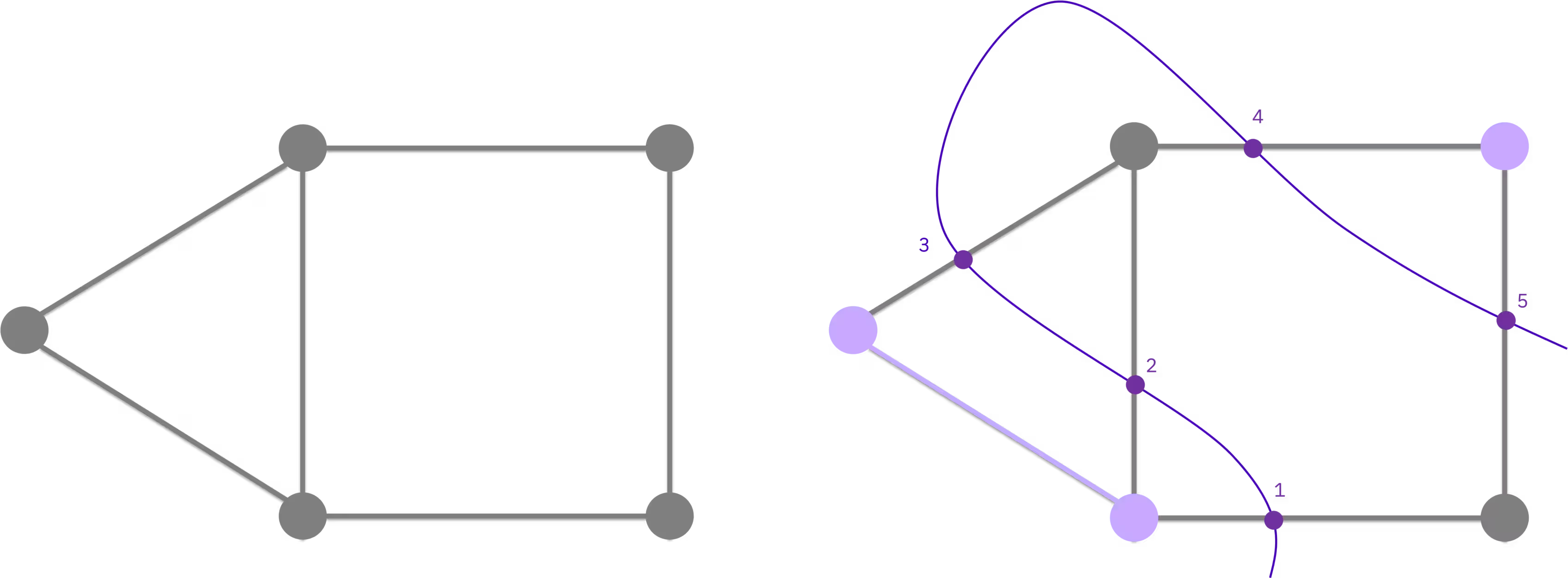
"**양자 근사 최적화 알고리즘(QAOA)** 은 조합 최적화 문제를 해결하기 위한 양자-고전 하이브리드 반복법이다. 이 튜토리얼에서는 QAOA를 사용하여 **최대 절단(max-cut)** 문제를 해결할 것입니다. 이 문제는 클러스터링, 네트워크 과학, 통계 물리학 등에 응용되는 NP-완전 최적화 문제입니다. 가장자리로 연결된 노드들로 구성된 그래프가 주어졌을 때, 분할을 가로지르는 가장자리의 개수가 최대가 되도록 노드들을 두 집합으로 나누는 것이 목표이다.\n",
"\n",
"\n",
"\n",
"\n",
"\n",
"### 고전 최적화에서 양자 회로에 이르기까지\n",
"\n",
"맥스컷은 고전적인 이진 최적화 문제로 표현될 수 있다. 각 노드에는 자신이 속한 집합을 나타내는 이진 변수 $x_i \\in \\{0, 1\\}$ 가 할당됩니다. 목표는 양 끝점이 서로 다른 집합에 속하는 변의 개수를 최대화하는 것입니다:\n",
"\n",
"$$\n",
"\\max_{x \\in \\{0,1\\}^n} \\sum_{(i,j)} x_i + x_j - 2x_ix_j.\n",
"$$\n",
"\n",
"이는 $\\min_x\\, x^T Q x$ 형태의 **2차 무제약 이진 최적화(QUBO)** 문제와 동등합니다. 표준 변수 대입( $x_i \\to (1 - Z_i)/2$ )을 통해, 이 QUBO는 기저 상태가 최적 해를 포함하는 **비용 해밀토니안** 으로 다시 표현될 수 있습니다. 일반적으로 이 해밀토니안은 2차 항과 1차 항을 모두 포함합니다:\n",
"\n",
"$$\n",
"H_C = \\sum_{ij} Q_{ij} \\, Z_i Z_j + \\sum_i b_i \\, Z_i.\n",
"$$\n",
"\n",
"여기서 다루는 가중치 없는 최대 절단 문제(unweighted max-cut problem)의 경우, 각 변에 대해 선형 계수들은 0이 되며( $b_i = 0$ ), $Q_{ij} = 1$ 이므로, 아래 코드에서 구현하게 될 더 간단한 형태인 $H_C = \\sum_{(i,j) \\in E} Z_i Z_j$ 가 남게 됩니다. 위에서 언급한 더 일반적인 형태는 이 워크플로를 가중 그래프나 기타 QUBO로 표현 가능한 문제로 적용할 때 필요한 것입니다.\n",
"\n",
"\n",
"\n",
"### QAOA의 작동 원리\n",
"\n",
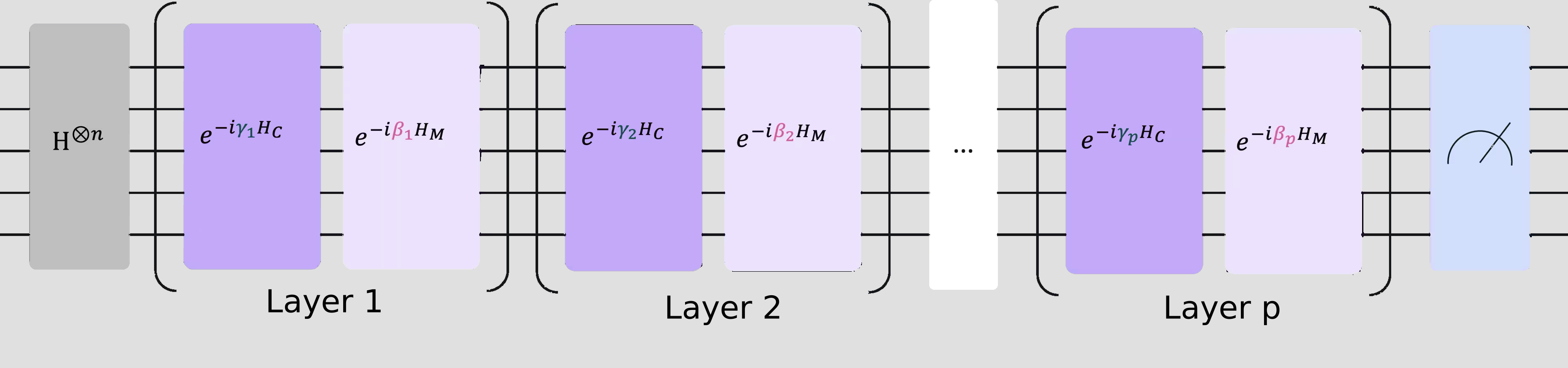
"QAOA는 초기 중첩 상태 $H^{\\otimes n}|0\\rangle$ 에 **비용** 연산자 $e^{-i\\gamma_k H_C}$ 와 **혼합** 연산자 $e^{-i\\beta_k H_m}$ 를 번갈아 가며 적용하여 후보 해를 도출합니다. 각도 $\\gamma_k$ 와 $\\beta_k$ 는 고전적 피드백 루프를 통해 최적화되며, 양자 컴퓨터는 비용 함수를 평가하고, 고전적 최적화기는 수렴할 때까지 매개변수를 업데이트합니다. 이 반복 루프는 양자 컴퓨팅 **세션** 내에서 실행되며, 이를 통해 반복 과정 전반에 걸쳐 양자 장치가 예약된 상태를 유지함으로써 지연 시간을 줄입니다.\n",
"\n",
"\n",
"\n",
"QUBO에서 해밀턴 연산자로의 완전한 유도 과정을 포함한 QAOA 이론에 대한 보다 심층적인 내용은 [QAOA 강의 모듈](/learning/courses/utility-scale-quantum-computing/variational-quantum-algorithms#1-introduction) 을 참고하십시오.\n",
"\n",
"이 튜토리얼에서는 먼저 5개 노드로 구성된 작은 그래프에서 최대 절단(max-cut) 문제를 해결한 다음, 실제 하드웨어 환경에서 동일한 워크플로를 100개 노드로 구성된 대규모 유틸리티급 문제로 확장해 보겠습니다. *요금제 이용 관련 참고 사항:* 이 튜토리얼에서는 ‘Quantum Compute’ [세션을](/docs/guides/execution-modes#session-mode) 사용하며, 이 세션은 프리미엄 요금제에서만 이용할 수 있습니다. Open Plan 요금제를 이용 중이라면, 이 튜토리얼을 설명된 대로 실행할 수 없습니다. 대신, `Session` 를 [작업](/docs/guides/execution-modes#job-mode) 모드로 변경해야 합니다(즉, 최적화 루프를 로 감싸지 않고 각 반복을 독립적인 작업으로 제출해야 합니다 `Session(...)`). 워크플로는 여전히 실행되지만, 각 반복마다 예약된 장치를 재사용하는 대신 전체 큐 지연 시간이 발생합니다. 자세한 내용은 [이용 가능한 요금제 개요를](/docs/guides/plans-overview) 참조하십시오.\n",
"\n"
]
},
{
"cell_type": "markdown",
"id": "381800e5",
"metadata": {},
"source": [
"\n",
"\n",
"## 요구사항\n",
"\n",
"이 튜토리얼을 시작하기 전에 다음이 설치되어 있는지 확인하세요:\n",
"\n",
"* Qiskit SDK v2.0 또는 그 이후 버전, [시각화](/docs/api/qiskit/visualization) 기능 지원\n",
"* Qiskit Runtime v0.22 또는 이후 (`pip install qiskit-ibm-runtime`)\n",
"\n",
"또한, [IBM Quantum® Platform](/docs/guides/cloud-setup) 에 있는 인스턴스에 접속할 수 있어야 합니다.\n",
"\n"
]
},
{
"cell_type": "markdown",
"id": "f5307376",
"metadata": {},
"source": [
"\n",
"\n",
"## 설정\n",
"\n"
]
},
{
"cell_type": "code",
"execution_count": 1,
"id": "37b3acfc",
"metadata": {},
"outputs": [],
"source": [
"import matplotlib.pyplot as plt\n",
"import rustworkx as rx\n",
"from rustworkx.visualization import mpl_draw as draw_graph\n",
"import numpy as np\n",
"from scipy.optimize import minimize\n",
"from collections import defaultdict\n",
"from typing import Sequence\n",
"\n",
"\n",
"from qiskit.quantum_info import SparsePauliOp\n",
"from qiskit.circuit.library import QAOAAnsatz\n",
"from qiskit.transpiler.preset_passmanagers import generate_preset_pass_manager\n",
"\n",
"from qiskit_ibm_runtime import QiskitRuntimeService\n",
"from qiskit_ibm_runtime import Session, EstimatorV2 as Estimator\n",
"from qiskit_ibm_runtime import SamplerV2 as Sampler"
]
},
{
"cell_type": "markdown",
"id": "68fd0b4f-baa4-45dc-9f4c-d9cdff01a651",
"metadata": {},
"source": [
"\n",
"\n",
"## 간단한 예시\n",
"\n",
"이 섹션에서는 5노드로 구성된 소규모 최대 절단(max-cut) 인스턴스를 예로 들어 QAOA 워크플로의 각 단계를 단계별로 설명합니다. “소규모”라는 표현이 붙었지만, 이 예제는 여전히 실제 IBM Quantum 하드웨어에서 실행됩니다. 코드는 127개 이상의 큐비트를 가진 백엔드를 선택하여 그곳에서 회로를 실행합니다.\n",
"\n"
]
},
{
"cell_type": "markdown",
"id": "0cbca6cb",
"metadata": {},
"source": [
"$n=5$ 노드로 그래프를 만들어 문제를 초기화합니다.\n",
"\n"
]
},
{
"cell_type": "code",
"execution_count": 2,
"id": "6ced6bea",
"metadata": {},
"outputs": [
{
"data": {
"text/plain": [
""
]
},
"metadata": {},
"output_type": "display_data"
}
],
"source": [
"n_small = 5\n",
"\n",
"graph = rx.PyGraph()\n",
"graph.add_nodes_from(np.arange(0, n_small, 1))\n",
"edge_list = [\n",
" (0, 1, 1.0),\n",
" (0, 2, 1.0),\n",
" (0, 4, 1.0),\n",
" (1, 2, 1.0),\n",
" (2, 3, 1.0),\n",
" (3, 4, 1.0),\n",
"]\n",
"graph.add_edges_from(edge_list)\n",
"draw_graph(graph, node_size=600, with_labels=True)"
]
},
{
"cell_type": "markdown",
"id": "a06e4386-d7bd-4914-9baa-36a5cc60e3ab",
"metadata": {},
"source": [
"\n",
"\n",
"### 1단계: 고전적 입력을 양자 문제에 매핑하기\n",
"\n",
"고전 그래프를 양자 **회로와** **연산자로** 매핑한다. [‘](#background) 배경’에서 설명한 바와 같이, 가중치 없는 최대 절단(unweighted max-cut)의 경우 비용 해밀토니안은 $H_C = \\sum_{(i,j) \\in E} Z_i Z_j$ 로 환원되며, QAOA는 매개변수화된 안잭 회로를 사용하여 $H_C$ 의 후보 기저 상태를 준비합니다.\n",
"\n"
]
},
{
"cell_type": "markdown",
"id": "a5b9e551-38a1-4543-b9f1-caaefb0ef3a9",
"metadata": {},
"source": [
"\n",
"\n",
"#### 비용 해밀토니안 구축\n",
"\n",
"그래프의 변을 파울리 $Z_iZ_j$ 항으로 변환하여 $H_C$ 를 구성한다(도출 과정은 [‘배경’](#background) 참조).\n",
"\n"
]
},
{
"cell_type": "code",
"execution_count": 3,
"id": "52d1ba92",
"metadata": {},
"outputs": [
{
"name": "stdout",
"output_type": "stream",
"text": [
"Cost Function Hamiltonian: SparsePauliOp(['IIIZZ', 'IIZIZ', 'ZIIIZ', 'IIZZI', 'IZZII', 'ZZIII'],\n",
" coeffs=[1.+0.j, 1.+0.j, 1.+0.j, 1.+0.j, 1.+0.j, 1.+0.j])\n"
]
}
],
"source": [
"def build_max_cut_paulis(\n",
" graph: rx.PyGraph,\n",
") -> list[tuple[str, list[int], float]]:\n",
" \"\"\"Convert graph edges to a list of ZZ Pauli terms.\n",
"\n",
" The returned list is in the sparse format expected by\n",
" ``SparsePauliOp.from_sparse_list``: each element is\n",
" ``(pauli_string, qubit_indices, coefficient)``.\n",
" \"\"\"\n",
" pauli_list = []\n",
" for edge in list(graph.edge_list()):\n",
" weight = graph.get_edge_data(edge[0], edge[1])\n",
" pauli_list.append((\"ZZ\", [edge[0], edge[1]], weight))\n",
" return pauli_list\n",
"\n",
"\n",
"max_cut_paulis = build_max_cut_paulis(graph)\n",
"cost_hamiltonian = SparsePauliOp.from_sparse_list(max_cut_paulis, n_small)\n",
"print(\"Cost Function Hamiltonian:\", cost_hamiltonian)"
]
},
{
"cell_type": "markdown",
"id": "33f71b0d-4a2a-4082-8c1a-ce9d2b769048",
"metadata": {},
"source": [
"\n",
"\n",
"#### QAOA 근사 회로 구축\n",
"\n"
]
},
{
"cell_type": "markdown",
"id": "00431c46-30c2-40f9-99df-40baf8da98f6",
"metadata": {},
"source": [
"를 `QAOAAnsatz` 사용하여 비용 해밀토니안으로부터 매개변수화된 QAOA 회로를 구성합니다. 여기서는 (두 개의 QAOA 층, 네 가지 매개변수: $\\beta_0, \\beta_1, \\gamma_0, \\gamma_1$ )를 사용합니다 `reps=2` .\n",
"\n"
]
},
{
"cell_type": "code",
"execution_count": 4,
"id": "7bd8c6d4-f40f-4a11-a440-0b26d9021b53",
"metadata": {},
"outputs": [
{
"data": {
"text/plain": [
""
]
},
"execution_count": 4,
"metadata": {},
"output_type": "execute_result"
}
],
"source": [
"circuit = QAOAAnsatz(cost_operator=cost_hamiltonian, reps=2)\n",
"circuit.measure_all()\n",
"\n",
"circuit.draw(\"mpl\")"
]
},
{
"cell_type": "code",
"execution_count": 5,
"id": "315c495a",
"metadata": {},
"outputs": [
{
"data": {
"text/plain": [
"ParameterView([ParameterVectorElement(β[0]), ParameterVectorElement(β[1]), ParameterVectorElement(γ[0]), ParameterVectorElement(γ[1])])"
]
},
"execution_count": 5,
"metadata": {},
"output_type": "execute_result"
}
],
"source": [
"circuit.parameters"
]
},
{
"cell_type": "markdown",
"id": "82f70daa-ff68-447a-8064-8b7df7a646cf",
"metadata": {},
"source": [
"\n",
"\n",
"### 2단계: 양자 하드웨어 실행을 위한 문제 최적화\n",
"\n"
]
},
{
"cell_type": "markdown",
"id": "c08be444-e3ed-4178-a10b-414069b1b411",
"metadata": {},
"source": [
"추상 회로를 하드웨어 전용 명령어로 변환한다. 이 단계에서는 큐비트 매핑, 게이트 분해, 라우팅 및 오류 억제를 처리합니다. 자세한 내용은 트랜스파일링 [문](/docs/guides/transpile) 서를 참조하십시오.\n",
"\n"
]
},
{
"cell_type": "code",
"execution_count": 6,
"id": "3f28a422-805c-4d3d-b5f6-62539e9133bd",
"metadata": {},
"outputs": [
{
"name": "stdout",
"output_type": "stream",
"text": [
"\n"
]
},
{
"data": {
"text/plain": [
""
]
},
"execution_count": 6,
"metadata": {},
"output_type": "execute_result"
}
],
"source": [
"service = QiskitRuntimeService()\n",
"backend = service.least_busy(\n",
" operational=True, simulator=False, min_num_qubits=127\n",
")\n",
"print(backend)\n",
"\n",
"# Create pass manager for transpilation. Level 3 is the most aggressive\n",
"# preset: slower to transpile, but produces shorter circuits that are\n",
"# more robust to hardware noise.\n",
"pm = generate_preset_pass_manager(optimization_level=3, backend=backend)\n",
"\n",
"candidate_circuit = pm.run(circuit)\n",
"candidate_circuit.draw(\"mpl\", fold=False, idle_wires=False)"
]
},
{
"cell_type": "markdown",
"id": "4e75cad7-f599-4937-b5fe-f4d01f53423c",
"metadata": {},
"source": [
"\n",
"\n",
"### 3단계: `Qiskit primitives` 명령어로 실행합니다\n",
"\n"
]
},
{
"cell_type": "markdown",
"id": "9b99ce67-f121-4244-b62a-536be38fea86",
"metadata": {},
"source": [
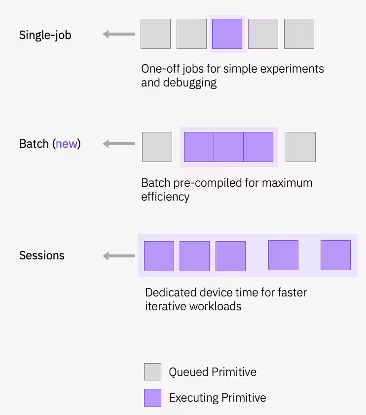
"QAOA 최적화 루프는 양자 컴퓨팅 [세션](/docs/guides/execution-modes) 내에서 실행되어, 반복 과정 전반에 걸쳐 장치가 예약된 상태를 유지합니다. 추정기는 각 단계에서 $\\langle H_C \\rangle$ 를 평가하며, 고전적 최적화기(COBYLA)는 수렴할 때까지 매개변수를 업데이트합니다.\n",
"\n",
"\n",
"\n"
]
},
{
"cell_type": "markdown",
"id": "00b2b0f1-9bad-4ad3-b93e-5cbf40395dbf",
"metadata": {},
"source": [
"초기 매개변수를 정의하고 최적화 루프를 실행합니다:\n",
"\n"
]
},
{
"cell_type": "code",
"execution_count": 7,
"id": "afa5747f-44dc-4e41-a875-7b6f896f13e2",
"metadata": {},
"outputs": [],
"source": [
"# QAOA doesn't prescribe principled default angles — any bounded choice\n",
"# works as a warm start for problems this small. beta and gamma are\n",
"# periodic (beta in [0, pi] and gamma in [0, 2*pi] modulo the underlying\n",
"# Pauli-rotation periods), and pi/2 and pi are just midpoints of those\n",
"# ranges. For harder problems you would typically warm start from known\n",
"# good angles or transfer parameters from smaller instances.\n",
"initial_gamma = np.pi\n",
"initial_beta = np.pi / 2\n",
"init_params = [initial_beta, initial_beta, initial_gamma, initial_gamma]"
]
},
{
"cell_type": "code",
"execution_count": 8,
"id": "3e64a862",
"metadata": {},
"outputs": [],
"source": [
"def cost_func_estimator(params, ansatz, hamiltonian, estimator):\n",
" # transform the observable defined on virtual qubits to\n",
" # an observable defined on all physical qubits\n",
" isa_hamiltonian = hamiltonian.apply_layout(ansatz.layout)\n",
"\n",
" pub = (ansatz, isa_hamiltonian, params)\n",
" job = estimator.run([pub])\n",
"\n",
" results = job.result()[0]\n",
" cost = results.data.evs\n",
"\n",
" objective_func_vals.append(cost)\n",
"\n",
" return cost"
]
},
{
"cell_type": "code",
"execution_count": 9,
"id": "2df241a9",
"metadata": {},
"outputs": [
{
"name": "stdout",
"output_type": "stream",
"text": [
" message: Return from COBYLA because the trust region radius reaches its lower bound.\n",
" success: True\n",
" status: 0\n",
" fun: -2.0402211719947774\n",
" x: [ 3.041e+00 1.212e+00 2.081e+00 4.471e+00]\n",
" nfev: 36\n",
" maxcv: 0.0\n"
]
}
],
"source": [
"objective_func_vals = [] # Global variable\n",
"with Session(backend=backend) as session:\n",
" # If using qiskit-ibm-runtime<0.24.0, change `mode=` to `session=`\n",
" estimator = Estimator(mode=session)\n",
" estimator.options.default_shots = 1000\n",
"\n",
" # Set simple error suppression/mitigation options\n",
" estimator.options.dynamical_decoupling.enable = True\n",
" estimator.options.dynamical_decoupling.sequence_type = \"XY4\"\n",
" estimator.options.twirling.enable_gates = True\n",
" estimator.options.twirling.num_randomizations = \"auto\"\n",
" estimator.options.environment.job_tags = [\"TUT_QAOA\"]\n",
"\n",
" result = minimize(\n",
" cost_func_estimator,\n",
" init_params,\n",
" args=(candidate_circuit, cost_hamiltonian, estimator),\n",
" method=\"COBYLA\",\n",
" tol=1e-2,\n",
" )\n",
" print(result)"
]
},
{
"cell_type": "markdown",
"id": "01d6b81c",
"metadata": {},
"source": [
"옵티마이저는 비용을 절감하고 회로의 더 나은 파라미터를 찾을 수 있었습니다.\n",
"\n",
"점차 완만하게 감소하다가 평탄해지는 곡선은 수렴의 특징이다. 시끄럽고 비단조적인 곡선은 대개 상류 단계에서 해결해야 할 문제가 있음을 나타냅니다. 일반적인 원인으로는 평가당 샘플 수가 너무 적거나(추정량의 분산이 큼), 초기 매개변수가 부적절하거나, 하드웨어 노이즈의 영향이 큰 회로 등이 있습니다. COBYLA는 미분 연산이 필요 없으며 중간 정도의 노이즈에 대해 상당히 견고하지만, 노이즈가 단계당 실제 비용 개선 효과를 압도하게 되면, 이 알고리즘의 선형 근사 모델은 더 이상 실제 하강과 무작위 변동을 구분하지 못하게 되어 최적화 과정이 방황하게 됩니다.\n",
"\n"
]
},
{
"cell_type": "code",
"execution_count": 10,
"id": "e14ecc92",
"metadata": {},
"outputs": [
{
"data": {
"text/plain": [
""
]
},
"metadata": {},
"output_type": "display_data"
}
],
"source": [
"plt.figure(figsize=(12, 6))\n",
"plt.plot(objective_func_vals)\n",
"plt.xlabel(\"Iteration\")\n",
"plt.ylabel(\"Cost\")\n",
"plt.show()"
]
},
{
"cell_type": "markdown",
"id": "1f9c8a9c",
"metadata": {},
"source": [
"최적화된 매개변수를 할당하고 Sampler 프리미티브를 사용하여 최종 분포를 샘플링합니다.\n",
"\n"
]
},
{
"cell_type": "code",
"execution_count": 11,
"id": "2989e76e-4296-4dd8-b065-2b8fced064cf",
"metadata": {},
"outputs": [
{
"data": {
"text/plain": [
""
]
},
"execution_count": 11,
"metadata": {},
"output_type": "execute_result"
}
],
"source": [
"optimized_circuit = candidate_circuit.assign_parameters(result.x)\n",
"optimized_circuit.draw(\"mpl\", fold=False, idle_wires=False)"
]
},
{
"cell_type": "code",
"execution_count": 12,
"id": "d8f0e302",
"metadata": {},
"outputs": [
{
"name": "stdout",
"output_type": "stream",
"text": [
"{18: 0.039, 5: 0.0665, 20: 0.0973, 29: 0.0063, 9: 0.0899, 13: 0.0379, 2: 0.0047, 1: 0.0153, 11: 0.0932, 14: 0.0327, 12: 0.0314, 25: 0.0193, 21: 0.0398, 6: 0.0224, 4: 0.0197, 10: 0.0387, 3: 0.0181, 26: 0.07, 17: 0.0327, 19: 0.0332, 22: 0.0914, 24: 0.007, 0: 0.0033, 8: 0.0066, 30: 0.0158, 28: 0.0169, 27: 0.0222, 16: 0.0073, 7: 0.0057, 23: 0.0062, 15: 0.0054, 31: 0.0041}\n"
]
}
],
"source": [
"# If using qiskit-ibm-runtime<0.24.0, change `mode=` to `backend=`\n",
"sampler = Sampler(mode=backend)\n",
"sampler.options.default_shots = 10000\n",
"\n",
"# Set simple error suppression/mitigation options\n",
"sampler.options.dynamical_decoupling.enable = True\n",
"sampler.options.dynamical_decoupling.sequence_type = \"XY4\"\n",
"sampler.options.twirling.enable_gates = True\n",
"sampler.options.twirling.num_randomizations = \"auto\"\n",
"\n",
"sampler.options.environment.job_tags = [\"TUT_QAOA\"]\n",
"\n",
"pub = (optimized_circuit,)\n",
"job = sampler.run([pub], shots=int(1e4))\n",
"counts_int = job.result()[0].data.meas.get_int_counts()\n",
"counts_bin = job.result()[0].data.meas.get_counts()\n",
"shots = sum(counts_int.values())\n",
"final_distribution_int = {key: val / shots for key, val in counts_int.items()}\n",
"final_distribution_bin = {key: val / shots for key, val in counts_bin.items()}\n",
"print(final_distribution_int)"
]
},
{
"cell_type": "markdown",
"id": "dace5fed-5555-4f1c-9109-7f5a31832d04",
"metadata": {},
"source": [
"\n",
"\n",
"### 4단계: 후처리 수행 및 원하는 클래식 형식으로 결과 반환\n",
"\n",
"표본 분포에서 가장 가능성이 높은 비트열을 추출한다. 이는 QAOA가 찾아낸 최상의 결과입니다.\n",
"\n"
]
},
{
"cell_type": "code",
"execution_count": 13,
"id": "d4f7fc70-883f-4b6b-8e92-2fc4afbbea46",
"metadata": {},
"outputs": [
{
"name": "stdout",
"output_type": "stream",
"text": [
"Result bitstring: [0, 0, 1, 0, 1]\n"
]
}
],
"source": [
"# auxiliary functions to sample most likely bitstring\n",
"def to_bitstring(integer, num_bits):\n",
" result = np.binary_repr(integer, width=num_bits)\n",
" return [int(digit) for digit in result]\n",
"\n",
"\n",
"keys = list(final_distribution_int.keys())\n",
"values = list(final_distribution_int.values())\n",
"most_likely = keys[np.argmax(np.abs(values))]\n",
"most_likely_bitstring = to_bitstring(most_likely, len(graph))\n",
"most_likely_bitstring.reverse()\n",
"\n",
"print(\"Result bitstring:\", most_likely_bitstring)"
]
},
{
"cell_type": "code",
"execution_count": 14,
"id": "650875e9-adbc-43bd-9505-556be2566278",
"metadata": {},
"outputs": [
{
"data": {
"text/plain": [
""
]
},
"metadata": {},
"output_type": "display_data"
}
],
"source": [
"plt.rcParams.update({\"font.size\": 10})\n",
"final_bits = final_distribution_bin\n",
"values = np.abs(list(final_bits.values()))\n",
"top_4_values = sorted(values, reverse=True)[:4]\n",
"positions = []\n",
"for value in top_4_values:\n",
" positions.append(np.where(values == value)[0])\n",
"fig = plt.figure(figsize=(11, 6))\n",
"ax = fig.add_subplot(1, 1, 1)\n",
"plt.xticks(rotation=45)\n",
"plt.title(\"Result Distribution\")\n",
"plt.xlabel(\"Bitstrings (reversed)\")\n",
"plt.ylabel(\"Probability\")\n",
"ax.bar(list(final_bits.keys()), list(final_bits.values()), color=\"tab:grey\")\n",
"for p in positions:\n",
" ax.get_children()[int(p[0])].set_color(\"tab:purple\")\n",
"plt.show()"
]
},
{
"cell_type": "markdown",
"id": "207443f2-34d9-424a-a6d7-44707ef1488b",
"metadata": {},
"source": [
"\n",
"\n",
"#### 최적 절단 시각화\n",
"\n",
"최적의 비트열을 바탕으로, 이 절단 부분을 원본 그래프에서 시각화할 수 있습니다.\n",
"\n"
]
},
{
"cell_type": "code",
"execution_count": 15,
"id": "33135970-8bc4-4fb2-ab87-08726a432ce4",
"metadata": {},
"outputs": [
{
"data": {
"text/plain": [
""
]
},
"metadata": {},
"output_type": "display_data"
}
],
"source": [
"# auxiliary function to plot graphs\n",
"def plot_result(G, x):\n",
" colors = [\"tab:grey\" if i == 0 else \"tab:purple\" for i in x]\n",
" pos, _default_axes = rx.spring_layout(G), plt.axes(frameon=True)\n",
" rx.visualization.mpl_draw(\n",
" G, node_color=colors, node_size=100, alpha=0.8, pos=pos\n",
" )\n",
"\n",
"\n",
"plot_result(graph, most_likely_bitstring)"
]
},
{
"cell_type": "markdown",
"id": "2119575f-f3cf-45bc-ae2b-93c046391eb6",
"metadata": {},
"source": [
"이제 절단면의 값을 계산해 봅시다:\n",
"\n"
]
},
{
"cell_type": "code",
"execution_count": 16,
"id": "2f6a73c4-f5ae-4647-a0dd-d77a13f66388",
"metadata": {},
"outputs": [
{
"name": "stdout",
"output_type": "stream",
"text": [
"The value of the cut is: 5\n"
]
}
],
"source": [
"def evaluate_sample(x: Sequence[int], graph: rx.PyGraph) -> float:\n",
" assert len(x) == len(\n",
" list(graph.nodes())\n",
" ), \"The length of x must coincide with the number of nodes in the graph.\"\n",
" return sum(\n",
" x[u] * (1 - x[v]) + x[v] * (1 - x[u])\n",
" for u, v in list(graph.edge_list())\n",
" )\n",
"\n",
"\n",
"cut_value = evaluate_sample(most_likely_bitstring, graph)\n",
"print(\"The value of the cut is:\", cut_value)"
]
},
{
"cell_type": "markdown",
"id": "76a7241e",
"metadata": {},
"source": [
"그래프가 이 정도로 작다면 진정한 최적 해를 무차별 대입법으로 쉽게 구할 수 있으므로, QAOA 결과를 정확한 정답과 비교하여 결과를 다시 확인할 수 있습니다.\n",
"\n"
]
},
{
"cell_type": "code",
"execution_count": 17,
"id": "0a3b5267",
"metadata": {},
"outputs": [
{
"name": "stdout",
"output_type": "stream",
"text": [
"Classical optimum (brute force): 5\n",
"QAOA cut value: 5\n"
]
}
],
"source": [
"# Classical baseline: enumerate all 2**n_small bitstrings and take the best cut.\n",
"def brute_force_max_cut(graph: rx.PyGraph) -> tuple[int, list[int]]:\n",
" n = len(list(graph.nodes()))\n",
" best_cut = -1\n",
" best_x: list[int] = []\n",
" for i in range(2**n):\n",
" x = [(i >> k) & 1 for k in range(n)]\n",
" cut = evaluate_sample(x, graph)\n",
" if cut > best_cut:\n",
" best_cut = int(cut)\n",
" best_x = x\n",
" return best_cut, best_x\n",
"\n",
"\n",
"classical_best, classical_x = brute_force_max_cut(graph)\n",
"print(f\"Classical optimum (brute force): {classical_best}\")\n",
"print(f\"QAOA cut value: {cut_value}\")"
]
},
{
"cell_type": "markdown",
"id": "large-scale-header",
"metadata": {},
"source": [
"\n",
"\n",
"## 대규모 하드웨어 예시\n",
"\n",
"IBM Quantum Platform 에서는 100 큐비트 이상의 용량을 갖춘 다양한 장치를 이용할 수 있습니다. 100개의 노드를 가진 가중 그래프에서 최대 절단 문제를 풀기 위해 하나를 선택하십시오. 이는 “대규모” 문제입니다. 이 워크플로는 위와 동일한 단계를 따르지만, 훨씬 더 큰 그래프에 적용됩니다.\n",
"\n"
]
},
{
"cell_type": "markdown",
"id": "large-scale-steps-intro",
"metadata": {},
"source": [
"\n",
"\n",
"### 대규모 유틸리티 수준의 종단간 워크플로\n",
"\n",
"100노드 그래프에 적용한 4단계의 전체 과정이 아래에 나와 있습니다. 구성은 소규모 예제와 동일합니다: 맵핑, 트랜스파일, 실행, 후처리 — 다만 문제 규모가 더 크며, 이해를 돕기 위해 아래의 네 개의 셀로 나누어 설명합니다.\n",
"\n"
]
},
{
"cell_type": "code",
"execution_count": null,
"id": "large-scale-helpers",
"metadata": {},
"outputs": [],
"source": [
"# Precomputed parity lookup table: _PARITY[b] = +1 if popcount(b) is even, else -1.\n",
"# We use this to vectorize expectation-value evaluation across all Pauli terms.\n",
"_PARITY = np.array(\n",
" [-1 if bin(i).count(\"1\") % 2 else 1 for i in range(256)],\n",
" dtype=np.complex128,\n",
")\n",
"\n",
"\n",
"def evaluate_sparse_pauli(state: int, observable: SparsePauliOp) -> complex:\n",
" \"\"\"Expectation value of a SparsePauliOp on a single computational-basis state.\n",
"\n",
" For a Z-only observable (which QAOA cost Hamiltonians are, after the\n",
" QUBO-to-Hamiltonian mapping), the eigenvalue of each Pauli term on a\n",
" computational-basis state is simply (-1)**popcount(z_mask AND state),\n",
" i.e., the parity of the bitwise-AND of the term's Z-support and the\n",
" measured bitstring.\n",
"\n",
" This routine packs the Z-support of every Pauli term into bytes, ANDs\n",
" them against the measured state in a single vectorized op, and looks up\n",
" the parity in _PARITY. For a 100-qubit / ~hundreds-of-terms Hamiltonian\n",
" over 10_000 samples, this is dramatically faster than calling\n",
" SparsePauliOp.expectation_value per sample.\n",
" \"\"\"\n",
" packed_uint8 = np.packbits(observable.paulis.z, axis=1, bitorder=\"little\")\n",
" state_bytes = np.frombuffer(\n",
" state.to_bytes(packed_uint8.shape[1], \"little\"), dtype=np.uint8\n",
" )\n",
" reduced = np.bitwise_xor.reduce(packed_uint8 & state_bytes, axis=1)\n",
" return np.sum(observable.coeffs * _PARITY[reduced])\n",
"\n",
"\n",
"def best_solution(samples, hamiltonian):\n",
" \"\"\"Return the sampled bitstring (as int) with the lowest Hamiltonian cost.\"\"\"\n",
" min_cost = float(\"inf\")\n",
" min_sol = None\n",
" for bit_str in samples.keys():\n",
" candidate_sol = int(bit_str)\n",
" fval = evaluate_sparse_pauli(candidate_sol, hamiltonian).real\n",
" if fval <= min_cost:\n",
" min_cost = fval\n",
" min_sol = candidate_sol\n",
" return min_sol\n",
"\n",
"\n",
"def _plot_cdf(objective_values: dict, ax, color):\n",
" x_vals = sorted(objective_values.keys(), reverse=True)\n",
" y_vals = np.cumsum([objective_values[x] for x in x_vals])\n",
" ax.plot(x_vals, y_vals, color=color)\n",
"\n",
"\n",
"def plot_cdf(dist, ax, title):\n",
" _plot_cdf(dist, ax, \"C1\")\n",
" ax.vlines(min(list(dist.keys())), 0, 1, \"C1\", linestyle=\"--\")\n",
" ax.set_title(title)\n",
" ax.set_xlabel(\"Objective function value\")\n",
" ax.set_ylabel(\"Cumulative distribution function\")\n",
" ax.grid(alpha=0.3)\n",
"\n",
"\n",
"def samples_to_objective_values(samples, hamiltonian):\n",
" \"\"\"Convert the samples to values of the objective function.\"\"\"\n",
" objective_values = defaultdict(float)\n",
" for bit_str, prob in samples.items():\n",
" candidate_sol = int(bit_str)\n",
" fval = evaluate_sparse_pauli(candidate_sol, hamiltonian).real\n",
" objective_values[fval] += prob\n",
" return objective_values"
]
},
{
"cell_type": "markdown",
"id": "4dc0c8ff",
"metadata": {},
"source": [
"**1단계** : 그래프, 비용 해밀토니안 및 가정을 수립한다.\n",
"\n"
]
},
{
"cell_type": "code",
"execution_count": 19,
"id": "94190344",
"metadata": {},
"outputs": [],
"source": [
"# Step 1: build the 100-node graph, cost Hamiltonian, and QAOA ansatz.\n",
"n_large = 100\n",
"graph_100 = rx.PyGraph()\n",
"graph_100.add_nodes_from(np.arange(0, n_large, 1))\n",
"elist = []\n",
"for edge in backend.coupling_map:\n",
" if edge[0] < n_large and edge[1] < n_large:\n",
" elist.append((edge[0], edge[1], 1.0))\n",
"graph_100.add_edges_from(elist)\n",
"\n",
"max_cut_paulis_100 = build_max_cut_paulis(graph_100)\n",
"cost_hamiltonian_100 = SparsePauliOp.from_sparse_list(\n",
" max_cut_paulis_100, n_large\n",
")\n",
"\n",
"circuit_100 = QAOAAnsatz(cost_operator=cost_hamiltonian_100, reps=1)\n",
"circuit_100.measure_all()"
]
},
{
"cell_type": "markdown",
"id": "c91f0c16",
"metadata": {},
"source": [
"**2단계** : 선택한 하드웨어 백엔드에 맞게 트랜스파일합니다.\n",
"\n"
]
},
{
"cell_type": "code",
"execution_count": 20,
"id": "2b59da0e",
"metadata": {},
"outputs": [],
"source": [
"# Step 2: transpile for hardware.\n",
"pm = generate_preset_pass_manager(optimization_level=3, backend=backend)\n",
"candidate_circuit_100 = pm.run(circuit_100)"
]
},
{
"cell_type": "markdown",
"id": "eb2c4d66",
"metadata": {},
"source": [
"**3단계** : 세션 내에서 QAOA 최적화 루프를 실행한 다음, 샘플링을 수행합니다.\n",
"\n"
]
},
{
"cell_type": "code",
"execution_count": 21,
"id": "e5aceab3",
"metadata": {},
"outputs": [
{
"name": "stdout",
"output_type": "stream",
"text": [
" message: Return from COBYLA because the trust region radius reaches its lower bound.\n",
" success: True\n",
" status: 0\n",
" fun: -17.172689238986344\n",
" x: [ 2.574e+00 4.166e+00]\n",
" nfev: 28\n",
" maxcv: 0.0\n"
]
}
],
"source": [
"# Step 3: run the QAOA optimization loop on the device, then sample the\n",
"# final distribution with the optimized parameters.\n",
"initial_gamma = np.pi\n",
"initial_beta = np.pi / 2\n",
"init_params = [initial_beta, initial_gamma]\n",
"\n",
"objective_func_vals = [] # Global variable\n",
"with Session(backend=backend) as session:\n",
" estimator = Estimator(mode=session)\n",
" estimator.options.default_shots = 1000\n",
"\n",
" # Set simple error suppression/mitigation options\n",
" estimator.options.dynamical_decoupling.enable = True\n",
" estimator.options.dynamical_decoupling.sequence_type = \"XY4\"\n",
" estimator.options.twirling.enable_gates = True\n",
" estimator.options.twirling.num_randomizations = \"auto\"\n",
" estimator.options.environment.job_tags = [\"TUT_QAOA\"]\n",
"\n",
" result = minimize(\n",
" cost_func_estimator,\n",
" init_params,\n",
" args=(candidate_circuit_100, cost_hamiltonian_100, estimator),\n",
" method=\"COBYLA\",\n",
" )\n",
" print(result)\n",
"\n",
"# Assign optimal parameters and sample the final distribution.\n",
"optimized_circuit_100 = candidate_circuit_100.assign_parameters(result.x)\n",
"\n",
"sampler = Sampler(mode=backend)\n",
"sampler.options.default_shots = 10000\n",
"\n",
"# Set simple error suppression/mitigation options\n",
"sampler.options.dynamical_decoupling.enable = True\n",
"sampler.options.dynamical_decoupling.sequence_type = \"XY4\"\n",
"sampler.options.twirling.enable_gates = True\n",
"sampler.options.twirling.num_randomizations = \"auto\"\n",
"\n",
"# Add a unique tag to the job execution\n",
"sampler.options.environment.job_tags = [\"TUT_QAOA\"]\n",
"\n",
"pub = (optimized_circuit_100,)\n",
"job = sampler.run([pub], shots=int(1e4))\n",
"\n",
"counts_int = job.result()[0].data.meas.get_int_counts()\n",
"shots = sum(counts_int.values())\n",
"final_distribution_100_int = {\n",
" key: val / shots for key, val in counts_int.items()\n",
"}"
]
},
{
"cell_type": "markdown",
"id": "7f0c5980",
"metadata": {},
"source": [
"**4단계** : 샘플링된 분포를 후처리하여 최적의 절단점을 추출합니다.\n",
"\n"
]
},
{
"cell_type": "code",
"execution_count": 22,
"id": "010571f7",
"metadata": {},
"outputs": [
{
"name": "stdout",
"output_type": "stream",
"text": [
"Result bitstring: [1, 1, 0, 1, 1, 0, 1, 1, 1, 0, 1, 0, 1, 1, 1, 0, 1, 1, 1, 1, 0, 0, 1, 0, 0, 1, 1, 0, 1, 0, 1, 0, 1, 1, 0, 1, 1, 0, 0, 0, 0, 0, 1, 1, 0, 1, 0, 0, 0, 1, 0, 0, 1, 0, 1, 0, 0, 1, 1, 1, 1, 1, 0, 1, 0, 1, 0, 0, 0, 1, 0, 1, 0, 1, 0, 0, 0, 0, 1, 0, 0, 1, 0, 1, 1, 1, 1, 0, 1, 0, 1, 0, 1, 1, 1, 0, 1, 1, 1, 0]\n",
"The value of the cut is: 156\n"
]
}
],
"source": [
"# Step 4: find the best-cost sample and evaluate its cut value.\n",
"best_sol_100 = best_solution(final_distribution_100_int, cost_hamiltonian_100)\n",
"best_sol_bitstring_100 = to_bitstring(int(best_sol_100), len(graph_100))\n",
"best_sol_bitstring_100.reverse()\n",
"\n",
"print(\"Result bitstring:\", best_sol_bitstring_100)\n",
"\n",
"cut_value_100 = evaluate_sample(best_sol_bitstring_100, graph_100)\n",
"print(\"The value of the cut is:\", cut_value_100)"
]
},
{
"cell_type": "markdown",
"id": "large-scale-convergence-md",
"metadata": {},
"source": [
"최적화 루프에서 최소화하려는 비용이 수렴했는지 확인하고, 결과를 시각화합니다.\n",
"\n"
]
},
{
"cell_type": "code",
"execution_count": 23,
"id": "large-scale-viz",
"metadata": {},
"outputs": [
{
"data": {
"text/plain": [
""
]
},
"metadata": {},
"output_type": "display_data"
},
{
"data": {
"text/plain": [
""
]
},
"metadata": {},
"output_type": "display_data"
},
{
"data": {
"text/plain": [
""
]
},
"metadata": {},
"output_type": "display_data"
}
],
"source": [
"# Plot convergence\n",
"plt.figure(figsize=(12, 6))\n",
"plt.plot(objective_func_vals)\n",
"plt.xlabel(\"Iteration\")\n",
"plt.ylabel(\"Cost\")\n",
"plt.show()\n",
"\n",
"# Visualize the cut\n",
"plot_result(graph_100, best_sol_bitstring_100)\n",
"\n",
"# Plot cumulative distribution function\n",
"result_dist = samples_to_objective_values(\n",
" final_distribution_100_int, cost_hamiltonian_100\n",
")\n",
"fig, ax = plt.subplots(1, 1, figsize=(8, 6))\n",
"plot_cdf(result_dist, ax, backend.name)"
]
},
{
"cell_type": "markdown",
"id": "69ebc85b-6a29-4671-8d16-1ac97f089607",
"metadata": {},
"source": [
"\n",
"\n",
"## 다음 단계\n",
"\n",
"이 글이 흥미로웠다면, 다음 자료도 참고해 보시기 바랍니다:\n",
"\n",
"\n",
" * [QAOA를 위한 고급 기법](/docs/tutorials/advanced-techniques-for-qaoa) — QAOA 성능 향상을 위한 고급 전략을 탐구한다\n",
" * [다목적 최적화 챌린지](https://github.com/qiskit-community/qdc-challenges-2025/blob/main/challenges/Track_B/qmoo/qmoo_qdc25.ipynb) — 다목적 양자 최적화를 주제로 한 이번 커뮤니티 챌린지에서 여러분의 실력을 시험해 보세요\n",
" * 회로 최적화 미세 조정을 위한 [트랜스파일레이션 문서](/docs/guides/transpile)\n",
" * 하드웨어 성능 향상을 위한 [오류 억제 및 완화](/docs/guides/error-mitigation-and-suppression-techniques)\n",
"\n",
"\n"
]
},
{
"cell_type": "markdown",
"metadata": {},
"id": "a1b8767d",
"source": "© IBM Corp., 2017-2026"
}
],
"metadata": {
"kernelspec": {
"display_name": "Python 3",
"language": "python",
"name": "python3"
},
"language_info": {
"codemirror_mode": {
"name": "ipython",
"version": 3
},
"file_extension": ".py",
"mimetype": "text/x-python",
"name": "python",
"nbconvert_exporter": "python",
"pygments_lexer": "ipython3",
"version": "3"
},
"hours": 1,
"qpuSeconds": 1320
},
"nbformat": 4,
"nbformat_minor": 5
}