{
"cells": [
{
"cell_type": "markdown",
"id": "e0cf0747",
"metadata": {},
"source": [
"---\n",
"title: \"変分量子アルゴリズム\"\n",
"description: \"このチュートリアルでは、ハイブリッド量子-古典アルゴリズムであるVQEとQAOAの概要を説明します\"\n",
"---\n",
"\n",
"\n",
"\n",
"# 量子アルゴリズム:変分量子アルゴリズム\n",
"\n",
"\n",
" 今道隆司(2024年5月24日)\n",
"\n",
" 講演の原文の [PDFをダウンロードする](https://ibm.ent.box.com/s/blnffu0pd7yzxarq3zc3w0jv90365ny2)。 これらは静的画像なので、いくつかのコード・スニペットは非推奨になるかもしれないことに注意してください。\n",
"\n",
" *この実験の実行にかかるQPU時間の目安は9分(Eagleプロセッサーでテスト)。*\n",
"\n",
" (このノートはオープン・プランの時間内に評価できないかもしれない)。 量子コンピューティングのリソースを賢く使ってください)\n",
"\n",
"\n"
]
},
{
"cell_type": "markdown",
"id": "59fbaadc",
"metadata": {},
"source": [
"\n",
"\n",
"## 1. はじめに\n",
"\n",
"このチュートリアルでは、特に変分量子固有値ソルバー(VQE)と量子近似最適化アルゴリズム(QAOA)に焦点を当て、ハイブリッド量子古典アルゴリズムの概要を説明します。 これらのアルゴリズムの主な目的は、パラメータ化された量子ゲートを持つ量子回路を用いて最適化問題に取り組むことである。\n",
"\n",
"量子コンピューティングの進歩にもかかわらず、現在の量子デバイスにはノイズが存在するため、深層量子回路から意味のある結果を引き出すことは困難である。 この課題を克服するため、VQEとQAOAは、量子計算で比較的短い量子回路を繰り返し実行し、古典計算で目標とするパラメトリック量子回路のパラメータを最適化するという、ハイブリッド量子古典アプローチを採用している。\n",
"\n",
"QAOAは、様々なエラー緩和・抑制技術の適用により、ユーティリティ・スケールで目標問題に対する最適解を提供する可能性を持っている。 VQEには(量子化学のように)スケーラビリティの低いアプリケーションも多い。 しかし、VQEを補完・補強するために、クリロフ部分空間対角化やサンプリングに基づく量子対角化(SQD)など、固有値に関連するアプローチが数多く登場している。 VQEを理解することは、登場した幅広い古典-量子ハイブリッドアルゴリズムを理解するための重要な第一歩である。\n",
"\n",
"このモジュールでは、VQEとQAOAの基本的なコンセプトと実装について説明する。 さらなるチュートリアルでは、これらのアルゴリズムをスケールアップするための高度なトピックとテクニックを探求する。\n",
"\n"
]
},
{
"cell_type": "markdown",
"id": "d3f4500f",
"metadata": {},
"source": [
"このノートブックを実行するには、以下のライブラリーが必要です。\n",
"まだインストールしていない場合は、コメントを外して以下のセルを実行すればインストールできる。\n",
"\n"
]
},
{
"cell_type": "code",
"execution_count": null,
"id": "2a8e650f",
"metadata": {},
"outputs": [],
"source": [
"# % pip install 'qiskit[visualization]' qiskit-ibm-runtime"
]
},
{
"cell_type": "markdown",
"id": "be601762",
"metadata": {},
"source": [
"\n",
"\n",
"## 2. 単純なハミルトニアンの最小固有値の計算\n",
"\n",
"まずは、VQEがどのように機能するのかを確認するために、非常にシンプルなケースにVQEを適用してみる。 VQEを用いてパウリ $Z$ 行列の最小固有値を計算する。 まずは一般的なパッケージをいくつかインポートする。\n",
"\n"
]
},
{
"cell_type": "code",
"execution_count": 1,
"id": "e8f398b2",
"metadata": {},
"outputs": [],
"source": [
"import numpy as np\n",
"from qiskit.circuit import ParameterVector, QuantumCircuit\n",
"from qiskit.primitives import StatevectorEstimator, StatevectorSampler\n",
"from qiskit.quantum_info import SparsePauliOp\n",
"from scipy.optimize import minimize"
]
},
{
"cell_type": "markdown",
"id": "d4395012",
"metadata": {},
"source": [
"ここで注目の演算子を定義し、行列形式で表示する。\n",
"\n"
]
},
{
"cell_type": "code",
"execution_count": 2,
"id": "a4f374a2",
"metadata": {},
"outputs": [
{
"data": {
"text/plain": [
"array([[ 1.+0.j, 0.+0.j],\n",
" [ 0.+0.j, -1.+0.j]])"
]
},
"execution_count": 2,
"metadata": {},
"output_type": "execute_result"
}
],
"source": [
"op = SparsePauliOp(\"Z\")\n",
"op.to_matrix()"
]
},
{
"cell_type": "markdown",
"id": "0a001e71",
"metadata": {},
"source": [
"古典的に固有値を求めるのは簡単なので、我々の作業をチェックすることができる。 これは、実用化に向けて規模を拡大するにつれて難しくなるかもしれない。 ここではnumpyを使う。\n",
"\n"
]
},
{
"cell_type": "code",
"execution_count": 3,
"id": "c9188662",
"metadata": {},
"outputs": [
{
"name": "stdout",
"output_type": "stream",
"text": [
"Eigenvalues: [-1. 1.]\n"
]
}
],
"source": [
"# compute eigenvalues with numpy\n",
"result = np.linalg.eigh(op.to_matrix())\n",
"print(\"Eigenvalues:\", result.eigenvalues)"
]
},
{
"cell_type": "markdown",
"id": "8f9af345",
"metadata": {},
"source": [
"変分量子アルゴリズムを使って固有値を求めるために、変分パラメータを取るゲートで回路を構成する:\n",
"\n"
]
},
{
"cell_type": "code",
"execution_count": 4,
"id": "99d5d36b",
"metadata": {},
"outputs": [
{
"data": {
"text/plain": [
""
]
},
"execution_count": 4,
"metadata": {},
"output_type": "execute_result"
}
],
"source": [
"# define a variational form\n",
"param = ParameterVector(\"a\", 3)\n",
"qc = QuantumCircuit(1, 1)\n",
"qc.u(param[0], param[1], param[2], 0)\n",
"qc_estimator = qc.copy()\n",
"qc.measure(0, 0)\n",
"qc.draw(\"mpl\")"
]
},
{
"cell_type": "markdown",
"id": "9607ab51",
"metadata": {},
"source": [
"ある演算子( $Z$ など)の期待値を推定したい場合は、Estimator を使用する。 システムの状態を見たい場合は、サンプラーを使う。\n",
"\n"
]
},
{
"cell_type": "code",
"execution_count": 5,
"id": "df8ed8d3",
"metadata": {},
"outputs": [],
"source": [
"sampler = StatevectorSampler()\n",
"estimator = StatevectorEstimator()"
]
},
{
"cell_type": "markdown",
"id": "880bccfb",
"metadata": {},
"source": [
"Samplerを使って、ビット列0と1のカウントをランダムなパラメータ値 `[1, 2, 3]` 。\n",
"\n"
]
},
{
"cell_type": "code",
"execution_count": 6,
"id": "5301ee71",
"metadata": {},
"outputs": [
{
"data": {
"text/plain": [
"{'0': 783, '1': 241}"
]
},
"execution_count": 6,
"metadata": {},
"output_type": "execute_result"
}
],
"source": [
"# compute counts of bitstrings with random parameter values by Sampler\n",
"result = sampler.run([(qc, [1, 2, 3])]).result()\n",
"counts = result[0].data.c.get_counts()\n",
"counts"
]
},
{
"cell_type": "markdown",
"id": "30ef9b8f",
"metadata": {},
"source": [
"Z の期待値は、確率 $\\{0: p_0, 1: p_1\\}$ を用いて $\\langle Z \\rangle = p_0 - p_1$ で計算できることがわかっている。\n",
"\n"
]
},
{
"cell_type": "code",
"execution_count": 7,
"id": "0f220c8d",
"metadata": {},
"outputs": [
{
"data": {
"text/plain": [
"0.529296875"
]
},
"execution_count": 7,
"metadata": {},
"output_type": "execute_result"
}
],
"source": [
"# compute the expectation value of Z based on the counts\n",
"(counts.get(\"0\", 0) - counts.get(\"1\", 0)) / sum(counts.values())"
]
},
{
"cell_type": "markdown",
"id": "695ee4bd",
"metadata": {},
"source": [
"この回路は機能したが、選ばれたパラメータ値は、非常に低エネルギー(あるいは低固有値)状態には対応しなかった。 得られた固有値は、最小値よりもかなり高い。 estimatorを使っても結果は同様である。\n",
"\n",
"なお、エスティメーターは測定なしで量子回路を作る。\n",
"\n"
]
},
{
"cell_type": "code",
"execution_count": 8,
"id": "c9e05530",
"metadata": {},
"outputs": [
{
"data": {
"text/plain": [
"array(0.54030231)"
]
},
"execution_count": 8,
"metadata": {},
"output_type": "execute_result"
}
],
"source": [
"result = estimator.run([(qc_estimator, op, [1, 2, 3])]).result()\n",
"result[0].data.evs"
]
},
{
"cell_type": "markdown",
"id": "b538e8b5",
"metadata": {},
"source": [
"パラメータを検索し、最小固有値をもたらすものを見つける必要がある。\n",
"変分形式のパラメータ値を受け取り、期待値 $\\langle Z \\rangle$ を返す関数を作る。\n",
"\n"
]
},
{
"cell_type": "code",
"execution_count": 9,
"id": "97fead46",
"metadata": {},
"outputs": [],
"source": [
"# define a cost function to look for the minimum eigenvalue of Z\n",
"def cost(x):\n",
" result = sampler.run([(qc, x)]).result()\n",
" counts = result[0].data.c.get_counts()\n",
" expval = (counts.get(\"0\", 0) - counts.get(\"1\", 0)) / sum(counts.values())\n",
" # the following line shows the trajectory of the optimization\n",
" print(expval, counts)\n",
" return expval"
]
},
{
"cell_type": "markdown",
"id": "a97eaeba",
"metadata": {},
"source": [
"SciPy's `minimize` 関数を適用して、Zの固有値の最小値を求めてみよう。\n",
"\n"
]
},
{
"cell_type": "code",
"execution_count": 10,
"id": "44f56300",
"metadata": {},
"outputs": [
{
"name": "stdout",
"output_type": "stream",
"text": [
"1.0 {'0': 1024}\n",
"0.494140625 {'0': 765, '1': 259}\n",
"0.466796875 {'0': 751, '1': 273}\n",
"0.564453125 {'0': 801, '1': 223}\n",
"-0.4296875 {'1': 732, '0': 292}\n",
"-0.984375 {'1': 1016, '0': 8}\n",
"-0.8984375 {'1': 972, '0': 52}\n",
"-0.990234375 {'1': 1019, '0': 5}\n",
"-0.892578125 {'1': 969, '0': 55}\n",
"-0.986328125 {'1': 1017, '0': 7}\n",
"-0.861328125 {'1': 953, '0': 71}\n",
"-1.0 {'1': 1024}\n",
"-0.982421875 {'1': 1015, '0': 9}\n",
"-0.99609375 {'1': 1022, '0': 2}\n",
"-0.986328125 {'1': 1017, '0': 7}\n",
"-1.0 {'1': 1024}\n",
"-0.990234375 {'1': 1019, '0': 5}\n",
"-0.998046875 {'1': 1023, '0': 1}\n",
"-0.99609375 {'1': 1022, '0': 2}\n",
"-1.0 {'1': 1024}\n",
"-1.0 {'1': 1024}\n",
"-1.0 {'1': 1024}\n",
"-1.0 {'1': 1024}\n",
"-0.998046875 {'1': 1023, '0': 1}\n",
"-1.0 {'1': 1024}\n",
"-1.0 {'1': 1024}\n",
"-0.998046875 {'1': 1023, '0': 1}\n",
"-0.998046875 {'1': 1023, '0': 1}\n",
"-0.998046875 {'1': 1023, '0': 1}\n",
"-1.0 {'1': 1024}\n",
"-0.99609375 {'1': 1022, '0': 2}\n",
"-1.0 {'1': 1024}\n",
"-0.99609375 {'1': 1022, '0': 2}\n",
"-0.998046875 {'1': 1023, '0': 1}\n",
"-0.998046875 {'1': 1023, '0': 1}\n",
"-0.99609375 {'1': 1022, '0': 2}\n",
"-0.998046875 {'1': 1023, '0': 1}\n",
"-1.0 {'1': 1024}\n",
"-0.998046875 {'1': 1023, '0': 1}\n",
"-0.998046875 {'1': 1023, '0': 1}\n",
"-0.99609375 {'1': 1022, '0': 2}\n",
"-1.0 {'1': 1024}\n",
"-0.998046875 {'1': 1023, '0': 1}\n",
"-1.0 {'1': 1024}\n",
"-0.998046875 {'1': 1023, '0': 1}\n",
"-0.998046875 {'1': 1023, '0': 1}\n",
"-1.0 {'1': 1024}\n",
"-0.998046875 {'1': 1023, '0': 1}\n",
"-0.998046875 {'1': 1023, '0': 1}\n",
"-1.0 {'1': 1024}\n",
"-1.0 {'1': 1024}\n",
"-1.0 {'1': 1024}\n",
"-1.0 {'1': 1024}\n",
"-1.0 {'1': 1024}\n",
"-1.0 {'1': 1024}\n",
"-0.998046875 {'1': 1023, '0': 1}\n",
"-0.994140625 {'1': 1021, '0': 3}\n",
"-1.0 {'1': 1024}\n",
"-1.0 {'1': 1024}\n",
"-1.0 {'1': 1024}\n",
"-1.0 {'1': 1024}\n",
"-1.0 {'1': 1024}\n",
"-1.0 {'1': 1024}\n"
]
},
{
"data": {
"text/plain": [
" message: Optimization terminated successfully.\n",
" success: True\n",
" status: 1\n",
" fun: -1.0\n",
" x: [ 3.182e+00 1.338e+00 1.664e-01]\n",
" nfev: 63\n",
" maxcv: 0.0"
]
},
"execution_count": 10,
"metadata": {},
"output_type": "execute_result"
}
],
"source": [
"# minimize the cost function with scipy's minimize\n",
"min_result = minimize(cost, [0, 0, 0], method=\"COBYLA\", tol=1e-8)\n",
"min_result"
]
},
{
"cell_type": "code",
"execution_count": 11,
"id": "4198224e",
"metadata": {},
"outputs": [
{
"data": {
"text/plain": [
"{'0': 1, '1': 1023}"
]
},
"execution_count": 11,
"metadata": {},
"output_type": "execute_result"
}
],
"source": [
"# check counts of bitstrings with the optimal parameters\n",
"result = sampler.run([(qc, min_result.x)]).result()\n",
"result[0].data.c.get_counts()"
]
},
{
"cell_type": "markdown",
"id": "d4e77e29",
"metadata": {},
"source": [
"\n",
"\n",
"### 2.1 運動\n",
"\n",
"$Z \\otimes Z$ の最小固有値を VQE で計算する。\n",
"\n"
]
},
{
"cell_type": "code",
"execution_count": 12,
"id": "86a2d76d",
"metadata": {},
"outputs": [
{
"name": "stdout",
"output_type": "stream",
"text": [
"SparsePauliOp(['ZZ'],\n",
" coeffs=[1.+0.j])\n",
"[[ 1.+0.j 0.+0.j 0.+0.j 0.+0.j]\n",
" [ 0.+0.j -1.+0.j 0.+0.j 0.+0.j]\n",
" [ 0.+0.j 0.+0.j -1.+0.j 0.+0.j]\n",
" [ 0.+0.j 0.+0.j 0.+0.j 1.+0.j]]\n"
]
}
],
"source": [
"z2 = SparsePauliOp(\"ZZ\")\n",
"print(z2)\n",
"print(z2.to_matrix())"
]
},
{
"cell_type": "code",
"execution_count": 15,
"id": "76092648-3b28-442e-8319-8a8416e0c9d5",
"metadata": {},
"outputs": [],
"source": [
"# compute eigenvalues with numpy"
]
},
{
"cell_type": "code",
"execution_count": 16,
"id": "f92a23b5",
"metadata": {},
"outputs": [],
"source": [
"# define a variational form\n",
"# qc = ..."
]
},
{
"cell_type": "code",
"execution_count": 17,
"id": "496572fb",
"metadata": {
"scrolled": true
},
"outputs": [],
"source": [
"# compute counts of bitstrings with a random parameter values by Sampler\n",
"# result = sampler.run(...)\n",
"# result"
]
},
{
"cell_type": "code",
"execution_count": 18,
"id": "b4cad5d0",
"metadata": {},
"outputs": [],
"source": [
"# compute the expectation value of ZZ based on the counts"
]
},
{
"cell_type": "code",
"execution_count": 19,
"id": "5ce555fe",
"metadata": {},
"outputs": [],
"source": [
"# verify the expectation value of ZZ with Estimator"
]
},
{
"cell_type": "code",
"execution_count": 20,
"id": "c210c435",
"metadata": {},
"outputs": [],
"source": [
"# define a cost function to look for the minimum eigenvalue of ZZ\n",
"# def cost(x):\n",
"# expval = ...\n",
"# return expval"
]
},
{
"cell_type": "code",
"execution_count": 21,
"id": "a75f3303",
"metadata": {},
"outputs": [],
"source": [
"# minimize the cost function with scipy's minimize\n",
"# min_result = minimize(cost, [...], method=\"COBYLA\", tol=1e-8)\n",
"# min_result"
]
},
{
"cell_type": "code",
"execution_count": 22,
"id": "8c476943",
"metadata": {},
"outputs": [],
"source": [
"# check counts of bitstrings with the optimal parameter values\n",
"# result = sampler.run(qc, min_result.x).result()\n",
"# result"
]
},
{
"cell_type": "markdown",
"id": "b82ba33a",
"metadata": {},
"source": [
"\n",
"\n",
"#### 演習問題の解答\n",
"\n"
]
},
{
"cell_type": "markdown",
"id": "7f2e0a4e",
"metadata": {},
"source": [
"目的の演算子を定義し、それを行列形式で表示する。\n",
"\n"
]
},
{
"cell_type": "code",
"execution_count": 13,
"id": "a1f9d371",
"metadata": {},
"outputs": [
{
"name": "stdout",
"output_type": "stream",
"text": [
"SparsePauliOp(['ZZ'],\n",
" coeffs=[1.+0.j])\n",
"[[ 1.+0.j 0.+0.j 0.+0.j 0.+0.j]\n",
" [ 0.+0.j -1.+0.j 0.+0.j 0.+0.j]\n",
" [ 0.+0.j 0.+0.j -1.+0.j 0.+0.j]\n",
" [ 0.+0.j 0.+0.j 0.+0.j 1.+0.j]]\n"
]
}
],
"source": [
"z2 = SparsePauliOp(\"ZZ\")\n",
"print(z2)\n",
"print(z2.to_matrix())"
]
},
{
"cell_type": "markdown",
"id": "b123e9d9",
"metadata": {},
"source": [
"変分量子アルゴリズムを使って固有値を求めるために、変分パラメータを取るゲートで回路を構成する:\n",
"\n"
]
},
{
"cell_type": "code",
"execution_count": 14,
"id": "7d5e894a",
"metadata": {},
"outputs": [
{
"data": {
"text/plain": [
""
]
},
"execution_count": 14,
"metadata": {},
"output_type": "execute_result"
}
],
"source": [
"# define a variational form\n",
"param = ParameterVector(\"a\", 6)\n",
"qc = QuantumCircuit(2, 2)\n",
"qc.u(param[0], param[1], param[2], 0)\n",
"qc.u(param[3], param[4], param[5], 1)\n",
"qc_estimator = qc.copy()\n",
"qc.measure([0, 1], [0, 1])\n",
"qc.draw(\"mpl\")"
]
},
{
"cell_type": "markdown",
"id": "f1d86563",
"metadata": {},
"source": [
"ある演算子( $Z \\otimes Z$ など)の期待値を推定したい場合は、Estimator を使うことになる。 システムの状態を見たい場合は、サンプラーを使う。\n",
"\n"
]
},
{
"cell_type": "code",
"execution_count": 15,
"id": "e3bda5ff",
"metadata": {},
"outputs": [],
"source": [
"sampler = StatevectorSampler()\n",
"estimator = StatevectorEstimator()"
]
},
{
"cell_type": "code",
"execution_count": 16,
"id": "aeac09f7",
"metadata": {},
"outputs": [
{
"data": {
"text/plain": [
"{'10': 661, '11': 203, '01': 47, '00': 113}"
]
},
"execution_count": 16,
"metadata": {},
"output_type": "execute_result"
}
],
"source": [
"# compute counts of bitstrings with random parameter values by Sampler\n",
"result = sampler.run([(qc, [1, 2, 3, 4, 5, 6])]).result()\n",
"counts = result[0].data.c.get_counts()\n",
"counts"
]
},
{
"cell_type": "code",
"execution_count": 17,
"id": "c96acbdf",
"metadata": {},
"outputs": [
{
"data": {
"text/plain": [
"-0.3828125"
]
},
"execution_count": 17,
"metadata": {},
"output_type": "execute_result"
}
],
"source": [
"# compute the expectation value of ZZ based on the counts\n",
"(\n",
" counts.get(\"00\", 0)\n",
" - counts.get(\"01\", 0)\n",
" - counts.get(\"10\", 0)\n",
" + counts.get(\"11\", 0)\n",
") / sum(counts.values())"
]
},
{
"cell_type": "markdown",
"id": "d2cc2ed8",
"metadata": {},
"source": [
"この回路は機能したが、選ばれたパラメータ値は、非常に低エネルギー(あるいは低固有値)状態には対応しなかった。 得られた固有値は、最小値よりもかなり高い。 estimatorを使っても結果は同様である。\n",
"\n"
]
},
{
"cell_type": "code",
"execution_count": 18,
"id": "474b84c5",
"metadata": {},
"outputs": [
{
"data": {
"text/plain": [
"array(-0.35316516)"
]
},
"execution_count": 18,
"metadata": {},
"output_type": "execute_result"
}
],
"source": [
"# verify the expectation value of ZZ with Estimator\n",
"result = estimator.run([(qc_estimator, z2, [1, 2, 3, 4, 5, 6])]).result()\n",
"result[0].data.evs"
]
},
{
"cell_type": "markdown",
"id": "25f4a655",
"metadata": {},
"source": [
"パラメータを検索し、最小固有値をもたらすものを見つける必要がある。\n",
"\n"
]
},
{
"cell_type": "code",
"execution_count": 19,
"id": "f29322f3",
"metadata": {},
"outputs": [],
"source": [
"# define a cost function to look for the minimum eigenvalue of ZZ\n",
"def cost(x):\n",
" result = sampler.run([(qc, x)]).result()\n",
" counts = result[0].data.c.get_counts()\n",
" expval = (\n",
" counts.get(\"00\", 0)\n",
" - counts.get(\"01\", 0)\n",
" - counts.get(\"10\", 0)\n",
" + counts.get(\"11\", 0)\n",
" ) / sum(counts.values())\n",
" print(expval, counts)\n",
" return expval"
]
},
{
"cell_type": "code",
"execution_count": 20,
"id": "12d8ba03",
"metadata": {},
"outputs": [
{
"name": "stdout",
"output_type": "stream",
"text": [
"1.0 {'00': 1024}\n",
"0.578125 {'00': 808, '01': 216}\n",
"0.5234375 {'00': 780, '01': 244}\n",
"0.548828125 {'00': 793, '01': 231}\n",
"0.3515625 {'00': 637, '10': 164, '11': 55, '01': 168}\n",
"0.3359375 {'00': 638, '11': 46, '10': 174, '01': 166}\n",
"0.283203125 {'00': 602, '10': 181, '01': 186, '11': 55}\n",
"-0.087890625 {'01': 414, '00': 184, '10': 143, '11': 283}\n",
"0.236328125 {'10': 27, '11': 623, '01': 364, '00': 10}\n",
"-0.0625 {'11': 261, '01': 403, '00': 219, '10': 141}\n",
"0.248046875 {'01': 366, '11': 628, '00': 11, '10': 19}\n",
"-0.0625 {'10': 145, '11': 254, '01': 399, '00': 226}\n",
"0.228515625 {'01': 373, '11': 609, '00': 20, '10': 22}\n",
"0.0546875 {'11': 376, '10': 273, '01': 211, '00': 164}\n",
"-0.447265625 {'01': 731, '10': 10, '11': 267, '00': 16}\n",
"-0.71484375 {'01': 871, '11': 99, '00': 47, '10': 7}\n",
"-0.46484375 {'01': 741, '00': 253, '10': 9, '11': 21}\n",
"-0.87890625 {'01': 962, '00': 39, '11': 23}\n",
"-0.640625 {'00': 176, '01': 837, '11': 8, '10': 3}\n",
"-0.88671875 {'01': 966, '00': 41, '11': 17}\n",
"-0.994140625 {'01': 1021, '11': 3}\n",
"-0.91796875 {'01': 982, '11': 35, '00': 7}\n",
"-0.994140625 {'01': 1021, '11': 2, '00': 1}\n",
"-0.939453125 {'01': 993, '00': 31}\n",
"-0.990234375 {'01': 1019, '11': 5}\n",
"-0.90234375 {'01': 974, '00': 21, '11': 29}\n",
"-0.98046875 {'01': 1014, '11': 10}\n",
"-0.994140625 {'01': 1021, '00': 3}\n",
"-0.990234375 {'01': 1019, '11': 4, '00': 1}\n",
"-0.98828125 {'01': 1018, '11': 6}\n",
"-0.990234375 {'01': 1019, '11': 4, '00': 1}\n",
"-0.994140625 {'01': 1021, '11': 2, '00': 1}\n",
"-0.99609375 {'01': 1022, '11': 2}\n",
"-0.998046875 {'01': 1023, '00': 1}\n",
"-0.99609375 {'01': 1022, '00': 2}\n",
"-1.0 {'01': 1024}\n",
"-1.0 {'01': 1024}\n",
"-1.0 {'01': 1024}\n",
"-0.998046875 {'01': 1023, '11': 1}\n",
"-1.0 {'01': 1024}\n",
"-1.0 {'01': 1024}\n",
"-1.0 {'01': 1024}\n",
"-1.0 {'01': 1024}\n",
"-1.0 {'01': 1024}\n",
"-1.0 {'01': 1024}\n",
"-1.0 {'01': 1024}\n",
"-0.998046875 {'01': 1023, '00': 1}\n",
"-0.998046875 {'01': 1023, '11': 1}\n",
"-0.998046875 {'01': 1023, '00': 1}\n",
"-1.0 {'01': 1024}\n",
"-1.0 {'01': 1024}\n",
"-1.0 {'01': 1024}\n",
"-1.0 {'01': 1024}\n",
"-1.0 {'01': 1024}\n",
"-1.0 {'01': 1024}\n",
"-0.998046875 {'01': 1023, '11': 1}\n",
"-0.998046875 {'01': 1023, '11': 1}\n",
"-1.0 {'01': 1024}\n",
"-1.0 {'01': 1024}\n",
"-0.998046875 {'01': 1023, '11': 1}\n",
"-0.998046875 {'01': 1023, '11': 1}\n",
"-0.998046875 {'01': 1023, '00': 1}\n",
"-1.0 {'01': 1024}\n",
"-1.0 {'01': 1024}\n",
"-0.998046875 {'01': 1023, '00': 1}\n",
"-1.0 {'01': 1024}\n",
"-1.0 {'01': 1024}\n",
"-1.0 {'01': 1024}\n",
"-1.0 {'01': 1024}\n",
"-0.998046875 {'01': 1023, '11': 1}\n",
"-0.998046875 {'01': 1023, '11': 1}\n",
"-1.0 {'01': 1024}\n",
"-0.998046875 {'01': 1023, '11': 1}\n",
"-1.0 {'01': 1024}\n",
"-1.0 {'01': 1024}\n",
"-1.0 {'01': 1024}\n",
"-0.998046875 {'01': 1023, '11': 1}\n",
"-0.998046875 {'01': 1023, '11': 1}\n",
"-1.0 {'01': 1024}\n",
"-1.0 {'01': 1024}\n",
"-0.998046875 {'01': 1023, '11': 1}\n",
"-0.998046875 {'01': 1023, '11': 1}\n",
"-0.998046875 {'01': 1023, '00': 1}\n",
"-1.0 {'01': 1024}\n",
"-1.0 {'01': 1024}\n",
"-1.0 {'01': 1024}\n",
"-0.998046875 {'01': 1023, '11': 1}\n",
"-1.0 {'01': 1024}\n",
"-0.99609375 {'01': 1022, '00': 1, '11': 1}\n",
"-0.998046875 {'01': 1023, '11': 1}\n",
"-0.998046875 {'01': 1023, '00': 1}\n",
"-0.998046875 {'01': 1023, '11': 1}\n",
"-1.0 {'01': 1024}\n",
"-0.99609375 {'01': 1022, '11': 1, '00': 1}\n",
"-1.0 {'01': 1024}\n",
"-0.998046875 {'01': 1023, '00': 1}\n",
"-0.994140625 {'01': 1021, '00': 3}\n",
"-0.998046875 {'01': 1023, '00': 1}\n",
"-0.99609375 {'01': 1022, '11': 2}\n",
"-1.0 {'01': 1024}\n",
"-1.0 {'01': 1024}\n",
"-0.998046875 {'01': 1023, '11': 1}\n",
"-1.0 {'01': 1024}\n",
"-1.0 {'01': 1024}\n",
"-1.0 {'01': 1024}\n",
"-1.0 {'01': 1024}\n",
"-1.0 {'01': 1024}\n",
"-1.0 {'01': 1024}\n",
"-0.998046875 {'01': 1023, '11': 1}\n",
"-1.0 {'01': 1024}\n",
"-1.0 {'01': 1024}\n",
"-1.0 {'01': 1024}\n",
"-0.998046875 {'01': 1023, '11': 1}\n",
"-0.998046875 {'01': 1023, '11': 1}\n",
"-1.0 {'01': 1024}\n",
"-0.998046875 {'01': 1023, '00': 1}\n",
"-1.0 {'01': 1024}\n",
"-1.0 {'01': 1024}\n",
"-1.0 {'01': 1024}\n",
"-1.0 {'01': 1024}\n",
"-1.0 {'01': 1024}\n",
"-1.0 {'01': 1024}\n",
"-0.998046875 {'01': 1023, '11': 1}\n",
"-0.998046875 {'01': 1023, '11': 1}\n",
"-0.998046875 {'01': 1023, '11': 1}\n",
"-0.99609375 {'01': 1022, '11': 2}\n",
"-1.0 {'01': 1024}\n",
"-0.998046875 {'01': 1023, '11': 1}\n"
]
},
{
"data": {
"text/plain": [
" message: Optimization terminated successfully.\n",
" success: True\n",
" status: 1\n",
" fun: -0.998046875\n",
" x: [ 3.167e+00 6.940e-01 1.033e+00 -2.894e-02 8.933e-01\n",
" 1.885e+00]\n",
" nfev: 128\n",
" maxcv: 0.0"
]
},
"execution_count": 20,
"metadata": {},
"output_type": "execute_result"
},
{
"data": {
"text/plain": [
" message: Optimization terminated successfully.\n",
" success: True\n",
" status: 1\n",
" fun: -0.99609375\n",
" x: [ 3.098e+00 -5.402e-01 1.091e+00 -1.004e-02 3.615e-01\n",
" 6.913e-01]\n",
" nfev: 115\n",
" maxcv: 0.0"
]
},
"execution_count": 30,
"metadata": {},
"output_type": "execute_result"
}
],
"source": [
"# minimize the cost function with scipy's minimize\n",
"min_result = minimize(cost, [0, 0, 0, 0, 0, 0], method=\"COBYLA\", tol=1e-8)\n",
"min_result"
]
},
{
"cell_type": "markdown",
"id": "d3e2de8d",
"metadata": {},
"source": [
"numpyから与えられた最小値に極めて近い固有値が得られた。\n",
"\n"
]
},
{
"cell_type": "code",
"execution_count": 21,
"id": "d34a8544",
"metadata": {},
"outputs": [
{
"data": {
"text/plain": [
"{'01': 1024}"
]
},
"execution_count": 21,
"metadata": {},
"output_type": "execute_result"
}
],
"source": [
"# check counts of bitstrings with the optimal parameters\n",
"result = sampler.run([(qc, min_result.x)]).result()\n",
"result[0].data.c.get_counts()"
]
},
{
"cell_type": "markdown",
"id": "bc51e7bf-e582-49ba-93f8-035624d56ccf",
"metadata": {},
"source": [
"\n",
"\n",
"## 3. Qiskitパターンを用いた量子最適化\n",
"\n",
"このハウツーでは、Qiskitパターンと量子近似最適化について学ぶ。 Qiskitパターンは、量子コンピューティングのワークフローを実装するための、直感的で反復可能なステップのセットです:\n",
"\n"
]
},
{
"attachments": {},
"cell_type": "markdown",
"id": "636ed1de-fc34-4cdd-9398-6fbd7c7fc9c6",
"metadata": {},
"source": [
"\n",
"\n"
]
},
{
"cell_type": "markdown",
"id": "8d3218ca-ce9e-40b4-a041-1b1d09bac8f5",
"metadata": {},
"source": [
"これらのパターンを**組み合わせ**最適化の文脈に適用し、ハイブリッド(量子・古典)反復法**である量子近似最適化アルゴリズム(QAOA)** を用いて**最大切断**問題を解く方法を示す。\n",
"\n",
"なお、このQAOAパートは、 [量子近似最適化アルゴリズム・](/docs/tutorials/quantum-approximate-optimization-algorithm) チュートリアルの「パート1:小規模QAOA」に基づいています。 拡大する方法はチュートリアルをご覧ください。\n",
"\n"
]
},
{
"cell_type": "markdown",
"id": "1e943b1a-218a-468c-bb63-4269896ebebe",
"metadata": {},
"source": [
"\n",
"\n",
"### 3.1 (小規模) 最適化のためのQiskitパターン\n",
"\n"
]
},
{
"cell_type": "markdown",
"id": "68fd0b4f-baa4-45dc-9f4c-d9cdff01a651",
"metadata": {},
"source": [
"このセクションでは、小規模な最大切断問題を用いて、量子コンピュータを用いて最適化問題を解くために必要な手順を説明します。\n",
"\n"
]
},
{
"cell_type": "markdown",
"id": "74b92ba5-c48a-405c-9c4b-04e985a7afbc",
"metadata": {},
"source": [
"最大カット問題は、クラスタリング、ネットワーク科学、統計物理学など、さまざまな分野で応用されているが、解くのが困難な最適化問題(より具体的には、NP困難問題)である。 このチュートリアルでは、辺で結ばれたノードからなるグラフを対象とし、辺を「切断」することでノードを2つの集合に分割し、切断される辺の数を最大化する方法を解説します。\n",
"\n"
]
},
{
"attachments": {},
"cell_type": "markdown",
"id": "887eb6ea-f58e-482f-8965-953a08fceecf",
"metadata": {},
"source": [
"\n",
"\n"
]
},
{
"cell_type": "markdown",
"id": "893a25f2",
"metadata": {},
"source": [
"この問題を量子アルゴリズムに適用する前に、背景を説明しておくと、まず関数 $f(x)$ の最小化について考えることで、最大切断問題がどのように古典的な組み合わせ最適化問題となるのかをよりよく理解できるでしょう\n",
"\n",
"$$\n",
"\\min_{x\\in \\{0, 1\\}^n}f(x),\n",
"$$\n",
"\n",
"ここで入力 $x$ は、グラフの各ノードに対応する成分を持つベクトルである。 次に、これらの各成分を $0$ または $1$ (カットに含まれるか含まれないかを表す)のいずれかになるように制約する。 この小規模な例では、 $n=5$ のノードを持つグラフを使用する。\n",
"\n",
"ノードのペア $i,j$、対応するエッジ $(i,j)$ がカット内にあるかどうかを示す関数を書くことができる。 例えば、関数 $x_i + x_j - 2 x_i x_j$ は、 $x_i$ と $x_j$ のどちらかが1の場合のみ1となり(これはエッジがカット内にあることを意味する)、それ以外は0となる。 カットのエッジを最大化する問題は次のように定式化できる\n",
"\n",
"$$\n",
"\\max_{x\\in \\{0, 1\\}^n} \\sum_{(i,j)} x_i + x_j - 2 x_i x_j,\n",
"$$\n",
"\n",
"の最小化として書き直すことができる\n",
"\n",
"$$\n",
"\\min_{x\\in \\{0, 1\\}^n} \\sum_{(i,j)} 2 x_i x_j - x_i - x_j.\n",
"$$\n",
"\n",
"この場合の $f(x)$ の最小値は、カットが横切る辺の数が最大になるときである。 ご覧の通り、量子コンピューティングに関連するものはまだ何もない。 この問題を量子コンピューターが理解できるように定式化する必要がある。\n",
"\n"
]
},
{
"cell_type": "markdown",
"id": "e2105a90-027f-44d7-97d1-c2c99373d488",
"metadata": {},
"source": [
"$n=5$ のノードでグラフを作成し、問題を初期化する。\n",
"\n"
]
},
{
"cell_type": "code",
"execution_count": 22,
"id": "d3c0dfa7",
"metadata": {},
"outputs": [],
"source": [
"import matplotlib\n",
"import matplotlib.pyplot as plt\n",
"import numpy as np\n",
"import rustworkx as rx\n",
"from rustworkx.visualization import mpl_draw"
]
},
{
"cell_type": "code",
"execution_count": 23,
"id": "99e763fe",
"metadata": {},
"outputs": [
{
"data": {
"text/plain": [
""
]
},
"metadata": {},
"output_type": "display_data"
}
],
"source": [
"n = 5\n",
"\n",
"graph = rx.PyGraph()\n",
"graph.add_nodes_from(range(1, n + 1))\n",
"edge_list = [\n",
" (0, 1, 1.0),\n",
" (0, 2, 1.0),\n",
" (1, 2, 1.0),\n",
" (1, 3, 1.0),\n",
" (2, 4, 1.0),\n",
" (3, 4, 1.0),\n",
"]\n",
"graph.add_edges_from(edge_list)\n",
"pos = rx.spring_layout(graph, seed=2)\n",
"mpl_draw(graph, node_size=600, pos=pos, with_labels=True, labels=str)"
]
},
{
"cell_type": "markdown",
"id": "a06e4386-d7bd-4914-9baa-36a5cc60e3ab",
"metadata": {},
"source": [
"\n",
"\n",
"### 3.2 ステップ1. 古典的な入力を量子問題にマッピングする\n",
"\n",
"このパターンの最初のステップは、古典的な問題(グラフ)を量子**回路と** **演算**子にマッピングすることである。 そのためには、主に3つのステップを踏む必要がある:\n",
"\n",
"1. 一連の数学的再定式化を利用し、2次制約なし2値最適化(QUBO)問題表記を用いてこの問題を表現する。\n",
"2. 最適化問題を、基底状態がコスト関数を最小化する解に対応するハミルトニアンとして書き直す。\n",
"3. 量子アニーリングに似たプロセスで、このハミルトニアンの基底状態を準備する量子回路を作る。\n",
"\n",
"**注:** QAOA手法では、最終的に、ハイブリッドアルゴリズムの**コスト関数を**表す演算子 (**ハミルトニアン** )と、問題の解の候補となる量子状態を表すパラメトライズ回路 (**アンサッツ** )を持ちたい。 これらの候補状態からサンプリングし、コスト関数を用いて評価することができる。\n",
"\n",
"\n",
"\n",
"#### グラフ → 最適化問題\n",
"\n",
"マッピングの最初のステップは表記法の変更である:\n",
"\n",
"$$\n",
"\\min_{x\\in \\{0, 1\\}^n}x^T Q x,\n",
"$$\n",
"\n",
"ここで、 $Q$ は実数の $n\\times n$ 行列、 $n$ はグラフのノード数、 $x$ は上で紹介したバイナリ変数のベクトル、 $x^T$ はベクトル $x$ の転置を示す。\n",
"\n"
]
},
{
"cell_type": "markdown",
"id": "c00a3493-abab-46d8-86a9-5b853979a575",
"metadata": {},
"source": [
"```\n",
"Problem name: maxcut\n",
"\n",
"Minimize\n",
" 2*x_1*x_2 + 2*x_1*x_3 + 2*x_2*x_3 + 2*x_2*x_4 + 2*x_3*x_5 + 2*x_4*x_5 - 2*x_1\n",
" - 3*x_2 - 3*x_3 - 2*x_4 - 2*x_5\n",
"\n",
"Subject to\n",
" No constraints\n",
"\n",
" Binary variables (5)\n",
" x_1 x_2 x_3 x_4 x_5\n",
"```\n",
"\n"
]
},
{
"cell_type": "markdown",
"id": "a5b9e551-38a1-4543-b9f1-caaefb0ef3a9",
"metadata": {},
"source": [
"\n",
"\n",
"#### 最適化問題 → ハミルトン量\n",
"\n",
"そして、QUBO問題を**ハミルトニアン** (ここでは系のエネルギーを表す行列)として再定式化することができる:\n",
"\n",
"$$\n",
"H_C=\\sum_{ij}Q_{ij}Z_iZ_j + \\sum_i b_iZ_i.\n",
"$$\n",
"\n",
"**QAOA問題からハミルトニアンへの再定式化ステップ**\n",
"\n",
"この方法でQAOA問題がどのように書き換えられるかを示すために、まず、バイナリ変数 $x_i$ を新しい変数セット $z_i\\in\\{-1, 1\\}$ に置き換える\n",
"\n",
"$$\n",
"x_i = \\frac{1-z_i}{2}.\n",
"$$\n",
"\n",
"ここで、 $x_i$ が $0$ であるならば、 $z_i$ は $1$ でなければならないことがわかる。 $x_i$ を最適化問題( $x^TQx$ )の $z_i$ に代入すると、等価な定式化が得られる。\n",
"\n",
"$$\n",
"x^TQx=\\sum_{ij}Q_{ij}x_ix_j \\\\ =\\frac{1}{4}\\sum_{ij}Q_{ij}(1-z_i)(1-z_j) \\\\=\\frac{1}{4}\\sum_{ij}Q_{ij}z_iz_j-\\frac{1}{4}\\sum_{ij}(Q_{ij}+Q_{ji})z_i + \\frac{n^2}{4}.\n",
"$$\n",
"\n",
"ここで、 $b_i=-\\sum_{j}(Q_{ij}+Q_{ji})$ を定義し、プレファクターと定数( $n^2$ )の項を取り除くと、同じ最適化問題の2つの等価な定式化に到達する。\n",
"\n",
"$$\n",
"min_{x\\in\\{0,1\\}^n} x^TQx\\Longleftrightarrow \\min_{z\\in\\{-1,1\\}^n}z^TQz + b^Tz\n",
"$$\n",
"\n",
"ここで、 $b$ は $Q$ に依存する。 $z^TQz + b^Tz$ を得るために、1/4 の係数と $n^2$ の定数オフセットを取り除いた。\n",
"\n",
"さて、問題の量子定式化を得るためには、 $z_i$ 変数を Pauli $Z$ 行列、例えば、 $2\\times 2$ 形式の行列に昇格させます\n",
"\n",
"$$\n",
"Z_i = \\begin{pmatrix}1 & 0 \\\\ 0 & -1\\end{pmatrix}.\n",
"$$\n",
"\n",
"これらの行列を上記の最適化問題に代入すると、次のようなハミルトニアンが得られる\n",
"\n",
"$$\n",
"H_C=\\sum_{ij}Q_{ij}Z_iZ_j + \\sum_i b_iZ_i.\n",
"$$\n",
"\n",
"*また、 $Z$ の行列は量子コンピュータの計算空間、つまりサイズ $2^n\\times 2^n$ のヒルベルト空間に埋め込まれていることを思い出してください。したがって、 $Z_iZ_j$ のような用語は、 $2^n\\times 2^n$ ヒルベルト空間に埋め込まれたテンソル積 $Z_i\\otimes Z_j$ として理解する必要があります。 例えば、5つの決定変数を持つ問題では、 $Z_1Z_3$ という用語は、 $I\\otimes Z_3\\otimes I\\otimes Z_1\\otimes I$ ( $I$ は $2\\times 2$ の恒等行列)を意味すると理解される。*\n",
"\n",
"このハミルトニアンは コスト関数ハミルトニアン と呼ばれ、その基底状態が はコスト関数 $f(x)$ の解に対応するという性質を持っています。 したがって、最適化問題を解くためには、 $H_C$ の基底状態(またはそれと重なりが大きい状態)を量子コンピュータに用意する必要があります。 そして、この状態からサンプリングすると、高い確率で $\\min~f(x)$ の解が得られる。\n",
"\n"
]
},
{
"cell_type": "code",
"execution_count": 24,
"id": "47256f53-8e02-494e-864a-a6f45b10442a",
"metadata": {},
"outputs": [],
"source": [
"def build_max_cut_operator(graph: rx.PyGraph) -> tuple[SparsePauliOp, float]:\n",
" sp_list = []\n",
" constant = 0\n",
" for s, t in graph.edge_list():\n",
" w = graph.get_edge_data(s, t)\n",
" sp_list.append((\"ZZ\", [s, t], w / 2))\n",
" constant -= 1 / 2\n",
" return SparsePauliOp.from_sparse_list(\n",
" sp_list, num_qubits=graph.num_nodes()\n",
" ), constant"
]
},
{
"cell_type": "code",
"execution_count": 25,
"id": "01a2d8eb-b63b-40bc-93c5-0b547c06b194",
"metadata": {},
"outputs": [
{
"name": "stdout",
"output_type": "stream",
"text": [
"Cost Function Hamiltonian: SparsePauliOp(['IIIZZ', 'IIZIZ', 'IIZZI', 'IZIZI', 'ZIZII', 'ZZIII'],\n",
" coeffs=[0.5+0.j, 0.5+0.j, 0.5+0.j, 0.5+0.j, 0.5+0.j, 0.5+0.j])\n",
"Constant: -3.0\n"
]
}
],
"source": [
"cost_hamiltonian, constant = build_max_cut_operator(graph)\n",
"print(\"Cost Function Hamiltonian:\", cost_hamiltonian)\n",
"print(\"Constant:\", constant)"
]
},
{
"cell_type": "markdown",
"id": "33f71b0d-4a2a-4082-8c1a-ce9d2b769048",
"metadata": {},
"source": [
"\n",
"\n",
"#### ハミルトニアン → 量子回路\n",
"\n"
]
},
{
"cell_type": "markdown",
"id": "00431c46-30c2-40f9-99df-40baf8da98f6",
"metadata": {},
"source": [
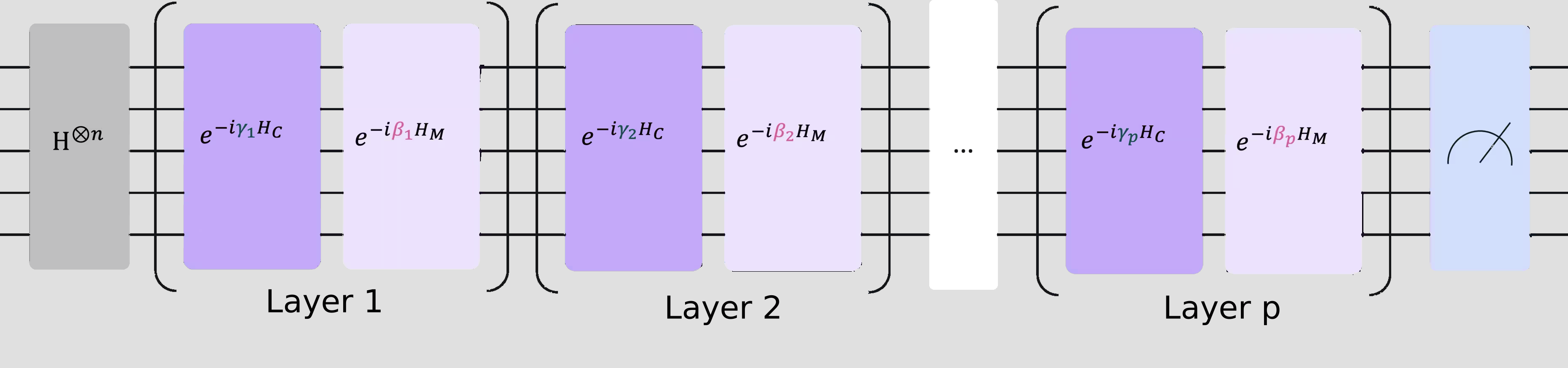
"ハミルトニアン $H_C$ には、あなたの問題の量子論的定義が含まれている。 これで、量子コンピューターから良い解を*サンプリングする*のに役立つ量子回路を作ることができる。 QAOAは量子アニーリングに着想を得ており、量子回路に演算子を交互に重ねて適用する。\n",
"\n",
"一般的な考え方は、既知のシステムの基底状態( $H^{\\otimes n}|0\\rangle$ )から始めて、興味のあるコスト演算子の基底状態にシステムを誘導することである。 これは、角度 $\\gamma_1,...,\\gamma_p$ と $\\beta_1,...,\\beta_p~$ を持つ演算子 $\\exp\\{-i\\gamma_k H_C\\}$ と $\\exp\\{-i\\beta_k H_m\\}$ を適用することによって行われる。\n",
"\n",
"生成される量子回路は、 $\\gamma_i$ と $\\beta_i$ で**パラメトリック化されて**いるので、 $\\gamma_i$ と $\\beta_i$ の異なる値を試して、結果の状態からサンプリングすることができます。\n",
"\n"
]
},
{
"attachments": {},
"cell_type": "markdown",
"id": "ca09d6bf-e421-4ada-9515-1f69687bb511",
"metadata": {},
"source": [
"\n",
"\n"
]
},
{
"cell_type": "markdown",
"id": "0d12bc53-7805-43e4-b4cb-754fd234b519",
"metadata": {},
"source": [
"今回は、 $\\gamma_1$ と $\\beta_1$ の2つのパラメーターを含む、1つのQAOAレイヤーの例を試してみる。\n",
"\n"
]
},
{
"cell_type": "code",
"execution_count": 26,
"id": "1f6215c0",
"metadata": {},
"outputs": [],
"source": [
"from qiskit.circuit.library import QAOAAnsatz"
]
},
{
"cell_type": "code",
"execution_count": 27,
"id": "7bd8c6d4-f40f-4a11-a440-0b26d9021b53",
"metadata": {},
"outputs": [
{
"data": {
"text/plain": [
""
]
},
"execution_count": 27,
"metadata": {},
"output_type": "execute_result"
}
],
"source": [
"circuit = QAOAAnsatz(cost_operator=cost_hamiltonian, reps=1)\n",
"circuit.measure_all()\n",
"circuit.draw(\"mpl\")"
]
},
{
"cell_type": "code",
"execution_count": 28,
"id": "148d2d62",
"metadata": {},
"outputs": [
{
"data": {
"text/plain": [
""
]
},
"execution_count": 28,
"metadata": {},
"output_type": "execute_result"
}
],
"source": [
"circuit.decompose(reps=3).draw(\"mpl\", fold=-1)"
]
},
{
"cell_type": "code",
"execution_count": 29,
"id": "315c495a",
"metadata": {},
"outputs": [
{
"data": {
"text/plain": [
"ParameterView([ParameterVectorElement(β[0]), ParameterVectorElement(γ[0])])"
]
},
"execution_count": 29,
"metadata": {},
"output_type": "execute_result"
}
],
"source": [
"circuit.parameters"
]
},
{
"cell_type": "markdown",
"id": "82f70daa-ff68-447a-8064-8b7df7a646cf",
"metadata": {},
"source": [
"\n",
"\n",
"### 3.3 ステップ2. 量子ハードウェア実行のための回路最適化\n",
"\n"
]
},
{
"cell_type": "markdown",
"id": "c08be444-e3ed-4178-a10b-414069b1b411",
"metadata": {},
"source": [
"上記の回路は、量子アルゴリズムを考えるのに便利な抽象化された一連の機能を含んでいるが、ハードウェア上で実行することは不可能である。 QPU上で動作させるためには、回路はパターンの**トランスパイルステップ**または**回路最適化**ステップを構成する一連の操作を受ける必要がある。\n",
"\n",
"Qiskitライブラリは、幅広い回路変換に対応する一連の**トランスピレーション・パスを**提供します。 回路が目的に応じて**最適化されて**いることを確認する必要がある。\n",
"\n",
"移籍には、次のようないくつかのステップがある:\n",
"\n",
"* 回路内の量子ビット(決定変数など)をデバイス上の物理量子ビットに**初期マッピング**する。\n",
"* 量子回路の命令を、バックエンドが理解できるハードウェアネイティブな命令に**アンロールする**。\n",
"* 相互作用する回路内のあらゆる量子ビットを、互いに隣接する物理量子ビットに**ルーティングする**。\n",
"* 動的デカップリングによるノイズ抑制のための単一量子ビットゲートの追加による**エラー抑制**。\n",
"\n",
"トランスピレーションの詳細については、 [ドキュメントを](/docs/guides/transpile)ご覧ください。\n",
"\n",
"以下のコードは、 **Qiskit IBM® Runtimeサービスを使って**、抽象回路をクラウド経由でアクセス可能なデバイスで実行可能な形式に変換し、最適化します。\n",
"\n",
"プログラムを実際の量子コンピュータに送る前に、\"ローカル・テスト・モード \"でローカルにテストすることができる。\n",
"ローカル・テスト・モードについての詳細は、 [ドキュメントを](/docs/guides/local-testing-mode)ご覧ください\n",
"\n"
]
},
{
"cell_type": "code",
"execution_count": null,
"id": "95cd3eed-0348-4373-b664-16a65d42f1e7",
"metadata": {},
"outputs": [
{
"name": "stderr",
"output_type": "stream",
"text": [
" service = QiskitRuntimeService(channel=\"ibm_quantum_platform\")\n"
]
},
{
"name": "stdout",
"output_type": "stream",
"text": [
"\n"
]
},
{
"data": {
"text/plain": [
""
]
},
"execution_count": 31,
"metadata": {},
"output_type": "execute_result"
}
],
"source": [
"from qiskit_ibm_runtime import QiskitRuntimeService\n",
"from qiskit.transpiler.preset_passmanagers import generate_preset_pass_manager\n",
"\n",
"# Use a quantum device\n",
"service = QiskitRuntimeService()\n",
"backend = service.least_busy(min_num_qubits=127)\n",
"# backend = service.backend(\"ibm_kingston\")\n",
"\n",
"# You can test your programs locally with a fake backend (local testing mode)\n",
"# backend = FakeBrisbane()\n",
"\n",
"print(backend)\n",
"\n",
"# Create pass manager for transpilation\n",
"pm = generate_preset_pass_manager(optimization_level=3, backend=backend)\n",
"\n",
"candidate_circuit = pm.run(circuit)\n",
"candidate_circuit.draw(\"mpl\", fold=False, idle_wires=False)"
]
},
{
"cell_type": "markdown",
"id": "4e75cad7-f599-4937-b5fe-f4d01f53423c",
"metadata": {},
"source": [
"\n",
"\n",
"### 3.4 ステップ3。 IBM Quantum プリミティブを使用して実行する\n",
"\n"
]
},
{
"cell_type": "markdown",
"id": "9b99ce67-f121-4244-b62a-536be38fea86",
"metadata": {},
"source": [
"QAOAワークフローでは、最適なQAOAパラメータは反復最適化ループで求められる。このループでは、一連の回路評価が実行され、古典的なオプティマイザを使用して最適な $\\beta_k$ および $\\gamma_k$ パラメータが求められる。 この実行ループは以下のステップを経て実行される:\n",
"\n",
"1. 初期パラメータの定義\n",
"2. 最適化ループと回路のサンプリングに使用したプリミティブを含む新しい `Session` をインスタンス化する\n",
"3. 最適なパラメータのセットが見つかったら、回路を最後に1回実行し、後処理ステップで使用する最終分布を得る。\n",
"\n"
]
},
{
"cell_type": "markdown",
"id": "00b2b0f1-9bad-4ad3-b93e-5cbf40395dbf",
"metadata": {},
"source": [
"\n",
"\n",
"#### 初期パラメータで回路を定義する\n",
"\n",
"任意に選んだパラメータでスタートする。\n",
"\n"
]
},
{
"cell_type": "code",
"execution_count": 32,
"id": "afa5747f-44dc-4e41-a875-7b6f896f13e2",
"metadata": {},
"outputs": [],
"source": [
"initial_gamma = np.pi\n",
"initial_beta = np.pi / 2\n",
"init_params = [initial_gamma, initial_beta]"
]
},
{
"cell_type": "markdown",
"id": "b867f1b0-7196-4d34-9b28-e3fb1de8221c",
"metadata": {},
"source": [
"\n",
"\n",
"#### バックエンドと実行プリミティブを定義する\n",
"\n",
"**IBM Quantum プリミティブ**を使用して、 IBM® バックエンドと連携します。 2つのプリミティブは「サンプラー」と「エスティメーター」であり、どのプリミティブを選択するかは、量子コンピュータ上でどのような測定を実行したいかによって決まります。 $H_C$ を最小化するには、コスト関数の値が単に $\\langle H_C \\rangle$ の期待値であるため、Estimator を使用します。\n",
"\n"
]
},
{
"cell_type": "markdown",
"id": "36c789f2",
"metadata": {},
"source": [
"\n",
"\n",
"#### 実行\n",
"\n",
"プリミティブは、量子デバイス上でワークロードをスケジューリングするための様々な[実行モードを](/docs/guides/execution-modes)提供し、QAOAワークフローはセッション内で繰り返し実行される。\n",
"\n"
]
},
{
"attachments": {},
"cell_type": "markdown",
"id": "122b7dc8-8d8a-45f2-813e-6199905d765b",
"metadata": {},
"source": [
"\n",
"\n"
]
},
{
"cell_type": "markdown",
"id": "fff58deb",
"metadata": {},
"source": [
"サンプラーベースのコスト関数を SciPy 最小化ルーチンに差し込むことで、最適なパラメーターを見つけることができる。\n",
"\n"
]
},
{
"cell_type": "code",
"execution_count": 33,
"id": "ff947109-cddc-4d3c-9119-2c729df73115",
"metadata": {},
"outputs": [],
"source": [
"def cost_func_estimator(params, ansatz, hamiltonian, estimator):\n",
" # transform the observable defined on virtual qubits to\n",
" # an observable defined on all physical qubits\n",
" isa_hamiltonian = hamiltonian.apply_layout(ansatz.layout)\n",
"\n",
" pub = (ansatz, isa_hamiltonian, params)\n",
" job = estimator.run([pub])\n",
"\n",
" results = job.result()[0]\n",
" cost = results.data.evs\n",
"\n",
" objective_func_vals.append(cost)\n",
"\n",
" return cost"
]
},
{
"cell_type": "code",
"execution_count": 34,
"id": "f5f46775",
"metadata": {},
"outputs": [
{
"name": "stdout",
"output_type": "stream",
"text": [
" message: Optimization terminated successfully.\n",
" success: True\n",
" status: 1\n",
" fun: -0.6557925874481715\n",
" x: [ 2.873e+00 9.414e-01]\n",
" nfev: 21\n",
" maxcv: 0.0\n"
]
}
],
"source": [
"from qiskit_ibm_runtime import Session, EstimatorV2\n",
"from scipy.optimize import minimize\n",
"\n",
"objective_func_vals = [] # Global variable\n",
"with Session(backend=backend) as session:\n",
" # If using qiskit-ibm-runtime<0.24.0, change `mode=` to `session=`\n",
" estimator = EstimatorV2(mode=session)\n",
" estimator.options.default_shots = 1000\n",
"\n",
" # Set simple error suppression/mitigation options\n",
" estimator.options.dynamical_decoupling.enable = True\n",
" estimator.options.dynamical_decoupling.sequence_type = \"XY4\"\n",
" estimator.options.twirling.enable_gates = True\n",
" estimator.options.twirling.num_randomizations = \"auto\"\n",
"\n",
" result = minimize(\n",
" cost_func_estimator,\n",
" init_params,\n",
" args=(candidate_circuit, cost_hamiltonian, estimator),\n",
" method=\"COBYLA\",\n",
" tol=1e-2,\n",
" )\n",
" print(result)"
]
},
{
"cell_type": "markdown",
"id": "ad878b62",
"metadata": {},
"source": [
"オプティマイザーは、コストを削減し、回路のより良いパラメータを見つけることができた。\n",
"\n"
]
},
{
"cell_type": "code",
"execution_count": 35,
"id": "f923dd5d",
"metadata": {},
"outputs": [
{
"data": {
"text/plain": [
""
]
},
"metadata": {},
"output_type": "display_data"
}
],
"source": [
"plt.figure(figsize=(12, 6))\n",
"plt.plot(objective_func_vals)\n",
"plt.xlabel(\"Iteration\")\n",
"plt.ylabel(\"Cost\")\n",
"plt.show()"
]
},
{
"cell_type": "markdown",
"id": "e2ea6359",
"metadata": {},
"source": [
"回路の最適なパラメータを見つけたら、これらのパラメータを割り当て、最適化されたパラメータで得られた最終分布をサンプリングすることができます。 グラフの最適カットに対応するビット列測定の確率分布であるため、ここで *Sampler* プリミティブを使用する。\n",
"\n",
"**注:** これは、コンピューター内に量子状態( $\\psi$ )を用意し、それを測定することを意味する。 測定は、状態を単一の計算基礎状態(例えば、 `010101110000...` )に折り畳む。これは、最初の最適化問題に対する解の候補 $x$ (タスクによっては $\\max f(x)$ または $\\min f(x)$ )に対応する。\n",
"\n"
]
},
{
"cell_type": "code",
"execution_count": 36,
"id": "f8dddf5a",
"metadata": {},
"outputs": [
{
"data": {
"text/plain": [
""
]
},
"execution_count": 36,
"metadata": {},
"output_type": "execute_result"
}
],
"source": [
"optimized_circuit = candidate_circuit.assign_parameters(result.x)\n",
"optimized_circuit.draw(\"mpl\", fold=False, idle_wires=False)"
]
},
{
"cell_type": "code",
"execution_count": 37,
"id": "fd9669cf",
"metadata": {},
"outputs": [
{
"name": "stdout",
"output_type": "stream",
"text": [
"{12: 0.0652, 31: 0.0089, 4: 0.0085, 13: 0.0731, 26: 0.0256, 28: 0.0246, 17: 0.0405, 25: 0.0591, 20: 0.031, 15: 0.0221, 8: 0.017, 21: 0.0371, 14: 0.0461, 16: 0.0229, 19: 0.0723, 23: 0.0199, 22: 0.0478, 18: 0.0708, 24: 0.0165, 6: 0.0525, 7: 0.0155, 5: 0.0245, 3: 0.0231, 29: 0.0121, 30: 0.0062, 10: 0.0363, 1: 0.0097, 9: 0.042, 27: 0.0094, 11: 0.0349, 0: 0.0129, 2: 0.0119}\n"
]
}
],
"source": [
"from qiskit_ibm_runtime import SamplerV2\n",
"\n",
"# If using qiskit-ibm-runtime<0.24.0, change `mode=` to `backend=`\n",
"sampler = SamplerV2(mode=backend)\n",
"\n",
"# Set simple error suppression/mitigation options\n",
"sampler.options.dynamical_decoupling.enable = True\n",
"sampler.options.dynamical_decoupling.sequence_type = \"XY4\"\n",
"sampler.options.twirling.enable_gates = True\n",
"sampler.options.twirling.num_randomizations = \"auto\"\n",
"\n",
"pub = (optimized_circuit,)\n",
"job = sampler.run([pub], shots=int(1e4))\n",
"counts_int = job.result()[0].data.meas.get_int_counts()\n",
"counts_bin = job.result()[0].data.meas.get_counts()\n",
"shots = sum(counts_int.values())\n",
"final_distribution_int = {key: val / shots for key, val in counts_int.items()}\n",
"final_distribution_bin = {key: val / shots for key, val in counts_bin.items()}\n",
"print(final_distribution_int)"
]
},
{
"cell_type": "markdown",
"id": "2c89613f",
"metadata": {},
"source": [
"\n",
"\n",
"### 3.5 ステップ4. 後処理を行い、結果を従来の形式で返す\n",
"\n",
"後処理ステップは、サンプリング出力を解釈して、元の問題の解を返す。 この場合、最も確率の高いビット列に興味があるはずだ。 問題の対称性によって、4つの解の可能性があり、サンプリング・プロセスはそのうちの1つを少し高い確率で返しますが、下のプロットされた分布では、4つのビット列が残りのビット列よりも明らかに可能性が高いことがわかります。\n",
"\n"
]
},
{
"cell_type": "code",
"execution_count": 38,
"id": "d4f7fc70-883f-4b6b-8e92-2fc4afbbea46",
"metadata": {},
"outputs": [
{
"name": "stdout",
"output_type": "stream",
"text": [
"Result bitstring: [1, 0, 1, 1, 0]\n"
]
}
],
"source": [
"# auxiliary functions to sample most likely bitstring\n",
"def to_bitstring(integer, num_bits):\n",
" result = np.binary_repr(integer, width=num_bits)\n",
" return [int(digit) for digit in result]\n",
"\n",
"\n",
"keys = list(final_distribution_int.keys())\n",
"values = list(final_distribution_int.values())\n",
"most_likely = keys[np.argmax(np.abs(values))]\n",
"most_likely_bitstring = to_bitstring(most_likely, len(graph))\n",
"most_likely_bitstring.reverse()\n",
"\n",
"print(\"Result bitstring:\", most_likely_bitstring)"
]
},
{
"cell_type": "code",
"execution_count": 39,
"id": "32a3020e-c1ea-4aff-988c-d7910a690fa8",
"metadata": {},
"outputs": [
{
"data": {
"text/plain": [
""
]
},
"metadata": {},
"output_type": "display_data"
}
],
"source": [
"import matplotlib.pyplot as plt\n",
"\n",
"matplotlib.rcParams.update({\"font.size\": 10})\n",
"final_bits = final_distribution_bin\n",
"values = np.abs(list(final_bits.values()))\n",
"top_4_values = sorted(values, reverse=True)[:4]\n",
"positions = []\n",
"for value in top_4_values:\n",
" positions.append(np.where(values == value)[0])\n",
"fig = plt.figure(figsize=(11, 6))\n",
"ax = fig.add_subplot(1, 1, 1)\n",
"plt.xticks(rotation=45)\n",
"plt.title(\"Result Distribution\")\n",
"plt.xlabel(\"Bitstrings (reversed)\")\n",
"plt.ylabel(\"Probability\")\n",
"ax.bar(list(final_bits.keys()), list(final_bits.values()), color=\"tab:grey\")\n",
"for p in positions:\n",
" ax.get_children()[p[0].item()].set_color(\"tab:purple\")\n",
"plt.show()"
]
},
{
"cell_type": "markdown",
"id": "6cfcb278",
"metadata": {},
"source": [
"\n",
"\n",
"#### 最適なカットを可視化する\n",
"\n",
"最適なビット列から、このカットを元のグラフ上に可視化することができる。\n",
"\n"
]
},
{
"cell_type": "code",
"execution_count": 40,
"id": "22a48124-e6b4-4144-bee1-f01fa4c7ccbb",
"metadata": {},
"outputs": [
{
"data": {
"text/plain": [
""
]
},
"metadata": {},
"output_type": "display_data"
}
],
"source": [
"colors = [\"tab:grey\" if i == 0 else \"tab:purple\" for i in most_likely_bitstring]\n",
"mpl_draw(graph, node_size=600, pos=pos, with_labels=True, labels=str, node_color=colors)"
]
},
{
"cell_type": "markdown",
"id": "4c4803ab",
"metadata": {},
"source": [
"そしてカットの価値を計算する。 ノイズのため最適解ではない(最適解のカット値は5)。\n",
"\n"
]
},
{
"cell_type": "code",
"execution_count": 41,
"id": "7208ee7d",
"metadata": {},
"outputs": [
{
"name": "stdout",
"output_type": "stream",
"text": [
"The value of the cut is: 5\n"
]
}
],
"source": [
"from typing import Sequence\n",
"\n",
"\n",
"def evaluate_sample(x: Sequence[int], graph: rx.PyGraph) -> float:\n",
" assert len(x) == len(\n",
" list(graph.nodes())\n",
" ), \"The length of x must coincide with the number of nodes in the graph.\"\n",
" return sum(\n",
" x[u] * (1 - x[v]) + x[v] * (1 - x[u]) for u, v in list(graph.edge_list())\n",
" )\n",
"\n",
"\n",
"cut_value = evaluate_sample(most_likely_bitstring, graph)\n",
"print(\"The value of the cut is:\", cut_value)"
]
},
{
"cell_type": "markdown",
"id": "1450be7e",
"metadata": {},
"source": [
"これで小規模のQAOAチュートリアルは終了。\n",
"QAOAをユーティリティ・スケールで適応させる方法は、\"パート2:スケールアップ!\"で学ぶことができる [量子近似最適化アルゴリズム](/docs/tutorials/quantum-approximate-optimization-algorithm)チュートリアルの\n",
"\n"
]
},
{
"cell_type": "code",
"execution_count": 42,
"id": "2a4f85ab",
"metadata": {},
"outputs": [
{
"data": {
"text/plain": [
"'2.0.2'"
]
},
"execution_count": 42,
"metadata": {},
"output_type": "execute_result"
}
],
"source": [
"# Check Qiskit version\n",
"import qiskit\n",
"\n",
"qiskit.__version__"
]
},
{
"cell_type": "markdown",
"metadata": {},
"id": "a1b8767d",
"source": "© IBM Corp., 2017-2026"
}
],
"metadata": {
"kernelspec": {
"display_name": "Python 3",
"language": "python",
"name": "python3"
},
"language_info": {
"codemirror_mode": {
"name": "ipython",
"version": 3
},
"file_extension": ".py",
"mimetype": "text/x-python",
"name": "python",
"nbconvert_exporter": "python",
"pygments_lexer": "ipython3",
"version": "3"
},
"widgets": {
"application/vnd.jupyter.widget-state+json": {
"state": {},
"version_major": 2,
"version_minor": 0
}
}
},
"nbformat": 4,
"nbformat_minor": 5
}