Bloch sphere

There's a useful geometric way to represent qubit states known as the Bloch sphere. It's very convenient, but unfortunately it only works for qubits — the analogous representation no longer corresponds to a spherical object once we have three or more classical states of our system.

---

Qubit states as points on a sphere

Let's start by thinking about a quantum state vector of a qubit: $\alpha \vert 0\rangle + \beta \vert 1\rangle.$ We can restrict our attention to vectors for which $\alpha$ is a nonnegative real number because every qubit state vector is equivalent up to a global phase to one for which $\alpha \geq 0.$ This allows us to write

$$\vert\psi\rangle = \cos\bigl(\theta/2\bigr) \vert 0\rangle + e^{i\phi} \sin\bigl(\theta/2\bigr) \vert 1\rangle$$

for two real numbers $\theta \in [0,\pi]$ and $\phi\in[0,2\pi).$ Here, we're allowing $\theta$ to range from $0$ to $\pi$ and dividing by $2$ in the argument of sine and cosine because this is a conventional way to parameterize vectors of this sort, and it will make things simpler a bit later on.

Now, it isn't quite the case that the numbers $\theta$ and $\phi$ are uniquely determined by a given quantum state vector $\alpha \vert 0\rangle + \beta \vert 1\rangle,$ but it is nearly so. In particular, if $\beta = 0,$ then $\theta = 0$ and it doesn't make any difference what value $\phi$ takes, so it can be chosen arbitrarily. Similarly, if $\alpha = 0,$ then $\theta = \pi,$ and once again $\phi$ is irrelevant (as our state is equivalent to $e^{i\phi}\vert 1\rangle$ for any $\phi$ up to a global phase). If, however, neither $\alpha$ nor $\beta$ is zero, then there's a unique choice for the pair $(\theta,\phi)$ for which $\vert\psi\rangle$ is equivalent to $\alpha\vert 0\rangle + \beta\vert 1\rangle$ up to a global phase.

Next, let's consider the density matrix representation of this state.

$$\vert\psi\rangle\langle\psi\vert = \begin{pmatrix} \cos^2(\theta/2) & e^{-i\phi}\cos(\theta/2)\sin(\theta/2)\\[2mm] e^{i\phi}\cos(\theta/2)\sin(\theta/2) & \sin^2(\theta/2) \end{pmatrix}$$

We can use some trigonometric identities,

$$\begin{gathered} \cos^2(\theta/2) = \frac{1 + \cos(\theta)}{2},\\[2mm] \sin^2(\theta/2) = \frac{1 - \cos(\theta)}{2},\\[2mm] \cos(\theta/2) \sin(\theta/2) = \frac{\sin(\theta)}{2}, \end{gathered}$$

as well as the formula $e^{i\phi} = \cos(\phi) + i\sin(\phi),$ to simplify the density matrix as follows.

$$\vert\psi\rangle\langle\psi\vert = \frac{1}{2} \begin{pmatrix} 1 + \cos(\theta) & (\cos(\phi) - i \sin(\phi)) \sin(\theta)\\[1mm] (\cos(\phi) + i \sin(\phi)) \sin(\theta) & 1 - \cos(\theta) \end{pmatrix}$$

This makes it easy to express this density matrix as a linear combination of the Pauli matrices:

$$\mathbb{I} = \begin{pmatrix} 1 & 0\\[1mm] 0 & 1 \end{pmatrix}, \quad \sigma_x = \begin{pmatrix} 0 & 1\\[1mm] 1 & 0 \end{pmatrix}, \quad \sigma_y = \begin{pmatrix} 0 & -i\\[1mm] i & 0 \end{pmatrix}, \quad \sigma_z = \begin{pmatrix} 1 & 0\\[1mm] 0 & -1 \end{pmatrix}.$$

Specifically, we conclude that

$$\vert\psi\rangle\langle\psi\vert = \frac{\mathbb{I} + \sin(\theta) \cos(\phi)\sigma_x + \sin(\theta)\sin(\phi) \sigma_y + \cos(\theta) \sigma_z}{2}.$$

The coefficients of $\sigma_x,$ $\sigma_y,$ and $\sigma_z$ in the numerator of this expression are all real numbers, so we can collect them together to form a vector in an ordinary, three-dimensional Euclidean space.

$$\bigl(\sin(\theta) \cos(\phi), \sin(\theta)\sin(\phi), \cos(\theta)\bigr)$$

In fact, this is a unit vector. Using spherical coordinates it can be written as $(1,\theta,\phi).$ The first coordinate, $1,$ represents the radius or radial distance (which is always $1$ in this case), $\theta$ represents the polar angle, and $\phi$ represents the azimuthal angle.

In words, thinking about a sphere as the planet Earth, the polar angle $\theta$ is how far we rotate south from the north pole to reach the point being described, from $0$ to $\pi = 180^{\circ},$ while the azimuthal angle $\phi$ is how far we rotate east from the prime meridian, from $0$ to $2\pi = 360^{\circ}.$ This assumes that we define the prime meridian to be the curve on the surface of the sphere from one pole to the other that passes through the positive $x$-axis.

Every point on the sphere can be described in this way — which is to say that the points we obtain when we range over all possible pure states of a qubit correspond precisely to a sphere in $3$ real dimensions. (This sphere is typically called the unit $2$-sphere because the surface of this sphere is two-dimensional.)

When we associate points on the unit $2$-sphere with pure states of qubits, we obtain the Bloch sphere representation these states.

---

Six important examples

1. The standard basis $\{\vert 0\rangle,\vert 1\rangle\}.$ Let's start with the state $\vert 0\rangle.$ As a density matrix it can be written like this.

   $$\vert 0 \rangle \langle 0 \vert = \frac{\mathbb{I} + \sigma_z}{2}$$

   By collecting the coefficients of the Pauli matrices in the numerator, we see that the corresponding point on the unit $2$-sphere using Cartesian coordinates is $(0,0,1).$ In spherical coordinates this point is $(1,0,\phi),$ where $\phi$ can be any angle. This is consistent with the expression

   $$\vert 0\rangle = \cos(0) \vert 0\rangle + e^{i \phi} \sin(0) \vert 1\rangle,$$

   which also works for any $\phi.$ Intuitively speaking, the polar angle $\theta$ is zero, so we're at the north pole of the Bloch sphere, where the azimuthal angle is irrelevant.

   Along similar lines, the density matrix for the state $\vert 1\rangle$ can be written like so.

   $$\vert 1 \rangle \langle 1 \vert = \frac{\mathbb{I} - \sigma_z}{2}$$

   This time the Cartesian coordinates are $(0,0,-1).$ In spherical coordinates this point is $(1,\pi,\phi)$ where $\phi$ can be any angle. In this case the polar angle is all the way to $\pi,$ so we're at the south pole where the azimuthal angle is again irrelevant.

2. The basis $\{\vert + \rangle, \vert - \rangle\}.$ We have these expressions for the density matrices corresponding to these states.

   $$\begin{aligned} \vert {+} \rangle\langle {+} \vert & = \frac{\mathbb{I} + \sigma_x}{2}\\[2mm] \vert {-} \rangle\langle {-} \vert & = \frac{\mathbb{I} - \sigma_x}{2} \end{aligned}$$

   The corresponding points on the unit $2$-sphere have Cartesian coordinates $(1,0,0)$ and $(-1,0,0),$ and spherical coordinates $(1,\pi/2,0)$ and $(1,\pi/2,\pi),$ respectively.

   In words, $\vert +\rangle$ corresponds to the point where the positive $x$-axis intersects the unit $2$-sphere and $\vert -\rangle$ corresponds to the point where the negative $x$-axis intersects it. More intuitively, $\vert +\rangle$ is on the equator of the Bloch sphere where it meets the prime meridian, and $\vert - \rangle$ is on the equator on the opposite side of the sphere.

3. The basis $\{\vert {+i} \rangle, \vert {-i} \rangle\}.$ As we saw earlier in the lesson, these two states are defined like this:

   $$\begin{aligned} \vert {+i} \rangle & = \frac{1}{\sqrt{2}} \vert 0 \rangle + \frac{i}{\sqrt{2}} \vert 1 \rangle\\[2mm] \vert {-i} \rangle & = \frac{1}{\sqrt{2}} \vert 0 \rangle - \frac{i}{\sqrt{2}} \vert 1 \rangle. \end{aligned}$$

   This time we have these expressions.

   $$\begin{aligned} \vert {+i} \rangle\langle {+i} \vert & = \frac{\mathbb{I} + \sigma_y}{2}\\[2mm] \vert {-i} \rangle\langle {-i} \vert & = \frac{\mathbb{I} - \sigma_y}{2} \end{aligned}$$

   The corresponding points on the unit $2$-sphere have Cartesian coordinates $(0,1,0)$ and $(0,-1,0),$ and spherical coordinates $(1,\pi/2,\pi/2)$ and $(1,\pi/2,3\pi/2),$ respectively.

   In words, $\vert {+i} \rangle$ corresponds to the point where the positive $y$-axis intersects the unit $2$-sphere and $\vert {-i} \rangle$ to the point where the negative $y$-axis intersects it.

Here's another class of quantum state vectors that has appeared from time to time throughout this series, including previously in this lesson.

$$\vert \psi_{\alpha} \rangle = \cos(\alpha) \vert 0\rangle + \sin(\alpha) \vert 1\rangle \qquad \text{(for $\alpha \in [0,\pi)$)}$$

The density matrix representation of each of these states is as follows.

$$\vert \psi_{\alpha} \rangle \langle \psi_{\alpha} \vert = \begin{pmatrix} \cos^2(\alpha) & \cos(\alpha)\sin(\alpha)\\[2mm] \cos(\alpha)\sin(\alpha) & \sin^2(\alpha) \end{pmatrix} = \frac{\mathbb{I} + \sin(2\alpha) \sigma_x + \cos(2\alpha) \sigma_z}{2}$$

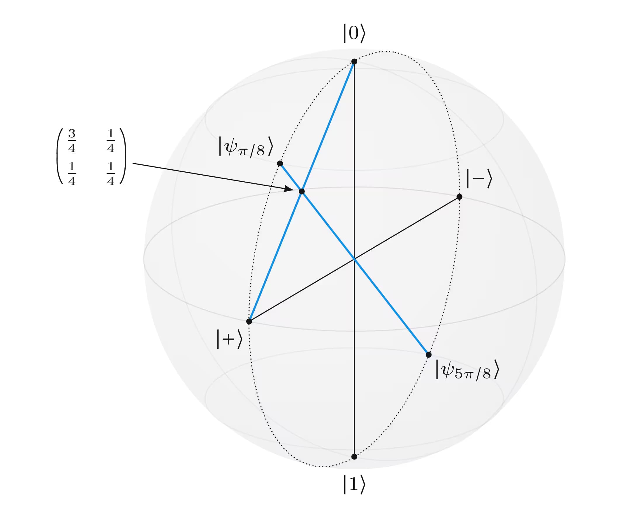
The following figure illustrates the corresponding points on the Bloch sphere for a few choices for $\alpha.$

---

Convex combinations of points

Similar to what we have already discussed for density matrices, we can take convex combinations of points on the Bloch sphere to obtain representations of qubit density matrices. In general, this results in points inside of the Bloch sphere, which represent density matrices of states that are not pure. Sometimes we refer to the Bloch ball when we wish to be explicit about the inclusion of points inside of the Bloch sphere as representations of qubit density matrices.

For example, we've seen that the density matrix $\frac{1}{2}\mathbb{I},$ which represents the completely mixed state of a qubit, can be written in these two alternative ways:

$$\frac{1}{2} \mathbb{I} = \frac{1}{2} \vert 0\rangle\langle 0\vert + \frac{1}{2} \vert 1\rangle\langle 1\vert \quad\text{and}\quad \frac{1}{2} \mathbb{I} = \frac{1}{2} \vert +\rangle\langle +\vert + \frac{1}{2} \vert -\rangle\langle -\vert.$$

We also have

$$\frac{1}{2} \mathbb{I} = \frac{1}{2} \vert {+i}\rangle\langle {+i} \vert + \frac{1}{2} \vert {-i} \rangle\langle {-i}\vert,$$

and more generally we can use any two orthogonal qubit state vectors (which will always correspond to two antipodal points on the Bloch sphere). If we average the corresponding points on the Bloch sphere in a similar way, we obtain the same point, which in this case is at the center of the sphere. This is consistent with the observation that

$$\frac{1}{2} \mathbb{I} = \frac{\mathbb{I} + 0 \cdot \sigma_x + 0 \cdot \sigma_y + 0 \cdot \sigma_z}{2},$$

giving us the Cartesian coordinates $(0,0,0).$

A different example concerning convex combinations of Bloch sphere points is the one discussed in the previous subsection.

$$\frac{1}{2} \vert 0\rangle\langle 0 \vert + \frac{1}{2} \vert +\rangle\langle + \vert = \begin{pmatrix} \frac{3}{4} & \frac{1}{4}\\[2mm] \frac{1}{4} & \frac{1}{4} \end{pmatrix} = \cos^2(\pi/8) \vert \psi_{\pi/8} \rangle \langle \psi_{\pi/8}\vert + \sin^2(\pi/8) \vert \psi_{5\pi/8} \rangle \langle \psi_{5\pi/8}\vert$$

The following figure illustrates these two different ways of obtaining this density matrix as a convex combination of pure states.