Quantum bits, gates, and circuits
Kifumi Numata (19 Apr 2024)
Click here to download the pdf of the original lecture. Note that some code snippets might become deprecated since these are static images.
Approximate QPU time to run this experiment is 5 seconds.
1. Introduction
Bits, gates, and circuits are the basic building blocks of quantum computing. You will learn quantum computation with the circuit model using quantum bits and gates, and also review the superposition, measurement, and entanglement.
In this lesson you will learn:
- Single-qubit gates
- Bloch sphere
- Superposition
- Measurement
- Two-qubit gates and entanglement state
At the end of this lecture, you will learn about circuit depth, which is essential for utility-scale quantum computing.
2. Computation as a diagram
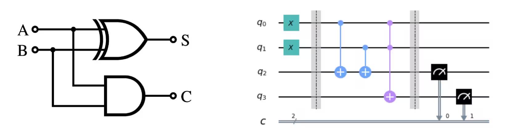
When using qubits or bits, we need to manipulate them in order to turn the inputs we have into the outputs we need. For the simplest programs with very few bits, it is useful to represent this process in a diagram known as a circuit diagram.
The bottom-left figure is an example of a classical circuit, and the bottom-right figure is an example of a quantum circuit. In both cases, the inputs are on the left and the outputs are on the right, while the operations are represented by symbols. The symbols used for the operations are called “gates”, mostly for historical reasons.
3. Single-qubit quantum gate
3.1 Quantum state and Bloch sphere
A qubit's state is represented as a superposition of and . An arbitrary quantum state is represented as
where and are complex numbers such that .
and are vectors in the two-dimensional complex vector space:
Therefore, an arbitrary quantum state is also represented as
From this, we can see that the state of a quantum bit is a unit vector in a two-dimensional complex inner product space with an orthonormal basis of and . It is normalized to 1.
is also called the statevector.
A single-qubit quantum state is also represented as
where and are the angles of the Bloch sphere in the following figure.

In the next few code cells, we will build up basic calculations from constituent pieces in Qiskit. We'll construct an empty circuit and then add quantum operations, discussing the gates and visualizing their effects as we go. You can run the cell by "Shift" + "Enter". Import the libraries first.
# Import the qiskit library
from qiskit import QuantumCircuit
from qiskit_aer import AerSimulator
from qiskit.quantum_info import Statevector
from qiskit.visualization import plot_bloch_multivector
from qiskit_ibm_runtime import Sampler
from qiskit.transpiler.preset_passmanagers import generate_preset_pass_manager
from qiskit.visualization import plot_histogram
Prepare the quantum circuit
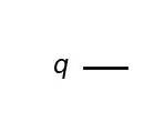
We will create and draw a single-qubit circuit.
# Create the single-qubit quantum circuit
qc = QuantumCircuit(1)

# Draw the circuit
qc.draw("mpl")
Output:
X gate
The X gate is a rotation around the axis of the Bloch sphere. Applying the X gate to results in , and applying the X gate to results in , so it is an operation similar to the classical NOT gate, and is also known as bit flip. The matrix representation of the X gate is below.
qc = QuantumCircuit(1)  # Prepare the single-qubit quantum circuit

# Apply a X gate to qubit 0
qc.x(0)

# Draw the circuit
qc.draw("mpl")
Output:

In IBM Quantum®, the initial state is set to , so the quantum circuit above in matrix representation is
Next, let's run this circuit using a statevector simulator.
# See the statevector
out_vector = Statevector(qc)
print(out_vector)
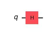
# Draw a Bloch sphere
plot_bloch_multivector(out_vector)Output:
Statevector([0.+0.j, 1.+0.j],
            dims=(2,))

Vertical vector is displayed as row vector, with complex numbers (the imaginary part is indexed by ).
H gate
The Hadamard gate is a rotation around an axis halfway between the and axes on the Bloch sphere. Applying the H gate to creates a superposition state such as . The matrix representation of the H gate is below.
qc = QuantumCircuit(1)  # Create the single-qubit quantum circuit

# Apply an Hadamard gate to qubit 0
qc.h(0)

# Draw the circuit
qc.draw(output="mpl")
Output:
# See the statevector
out_vector = Statevector(qc)
print(out_vector)

# Draw a Bloch sphere
plot_bloch_multivector(out_vector)
Output:
Statevector([0.70710678+0.j, 0.70710678+0.j],
            dims=(2,))
This is
This superposition state is so common and important, that it is given its own symbol:
By applying the gate on the , we created a superposition of and where measurement in the computational basis (along z in the Bloch sphere picture) would give you each state with equal probabilities.
state
You might have guessed that there is a corresponding state:
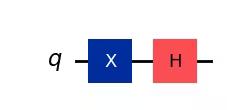
To create this state, first apply an X gate to make , then apply an H gate.
qc = QuantumCircuit(1)  # Create the single-qubit quantum circuit

# Apply a X gate to qubit 0
qc.x(0)

# Apply an Hadamard gate to qubit 0
qc.h(0)

# draw the circuit
qc.draw(output="mpl")
Output:
# See the statevector
out_vector = Statevector(qc)
print(out_vector)

# Draw a Bloch sphere
plot_bloch_multivector(out_vector)
Output:
Statevector([ 0.70710678+0.j, -0.70710678+0.j],
            dims=(2,))
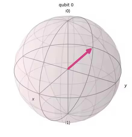
This is
Applying the gate on results in an equal superposition of and , but the sign of is negative.
3.2 Single-qubit quantum state and unitary evolution
The actions of all the gates we have seen so far have been unitary, which means they can be represented by a unitary operator. In other words, the output state can be obtained by acting on the initial state with a unitary matrix:
A unitary matrix is a matrix satisfying
In terms of quantum computer operation, we would say that applying a quantum gate to the qubit evolves the quantum state. Common single-qubit gates include the following.
Pauli gates:
where the outer product was calculated as follows:
Other typical single-qubit gates:
The meaning and use of these are described in more detail in the Basics of Quantum Information course.
Exercise 1
Use Qiskit to create quantum circuits that prepare the states described below. Then run each circuit using the statevector simulator and display the resulting state on the Bloch sphere. As a bonus, see if you can anticipate what the final state should be based on intuition about the gates and rotations in the Bloch sphere.
(1)
(2)
(3)
Tips: Z gate can be used by
qc.z(0)
Solution:
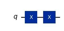
### (1) XX|0> ###

# Create the single-qubit quantum circuit
qc = QuantumCircuit(1)  ##your code goes here##

# Add a X gate to qubit 0
qc.x(0)  ##your code goes here##

# Add a X gate to qubit 0
qc.x(0)  ##your code goes here##

# Draw a circuit
qc.draw(output="mpl")
Output:
# See the statevector
out_vector = Statevector(qc)
print(out_vector)

# Draw a Bloch sphere
plot_bloch_multivector(out_vector)
Output:
Statevector([1.+0.j, 0.+0.j],
            dims=(2,))

### (2) HH|0> ###
##your code goes here##
qc = QuantumCircuit(1)
qc.h(0)
qc.h(0)
qc.draw("mpl")
Output:
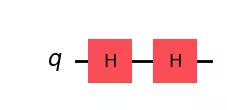
# See the statevector
out_vector = Statevector(qc)
print(out_vector)

# Draw a Bloch sphere
plot_bloch_multivector(out_vector)
Output:
Statevector([1.+0.j, 0.+0.j],
            dims=(2,))
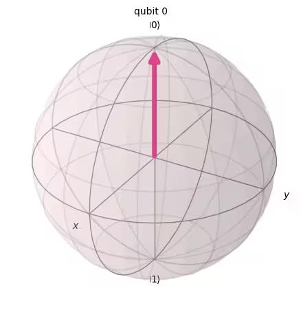
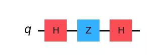
### (3) HZH|0> ###
##your code goes here##
qc = QuantumCircuit(1)
qc.h(0)
qc.z(0)
qc.h(0)
qc.draw("mpl")
Output:
# See the statevector
out_vector = Statevector(qc)
print(out_vector)
# Draw a Bloch sphere
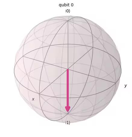
plot_bloch_multivector(out_vector)Output:
Statevector([0.+0.j, 1.+0.j],
            dims=(2,))
3.3 Measurement
Measurement is theoretically a very complicated topic. But in practical terms, making a measurement along (as all IBM® quantum computers do) simply forces the qubit’s state either to or to and we observe the outcome.
- is the probability we will get when we measure.
- is the probability we will get when we measure.
So, and are called probability amplitudes. (see "Born rule")
For example, has an equal probability of becoming or upon measurement. has a 75% chance of becoming .
Qiskit Aer Simulator
Next, let's measure a circuit that prepares the equal probability superposition above. We should add the measurement gates, as the Qiskit Aer simulator simulates an ideal (with no noise) quantum hardware by default. Note: The Aer simulator can also apply a noise model based on real quantum computer. We will return to noise models later.
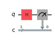
# Create a new circuit with one qubits (first argument) and one classical bits (second argument)
qc = QuantumCircuit(1, 1)
qc.h(0)
qc.measure(0, 0)  # Add the measurement gate

qc.draw(output="mpl")
Output:
We are now ready to run our circuit on the Aer simulator. In this example, we will apply the default shots=1024, which means we will measure 1024 times. Then we will plot those counts in a histogram.
# Run the circuit on a simulator to get the results
# Define backend
backend = AerSimulator()

# Transpile to backend
pm = generate_preset_pass_manager(backend=backend, optimization_level=1)
isa_qc = pm.run(qc)

# Run the job
sampler = Sampler(mode=backend)
job = sampler.run([isa_qc])
result = job.result()

# Print the results
counts = result[0].data.c.get_counts()
print(counts)

# Plot the counts in a histogram
plot_histogram(counts)
Output:
{'0': 521, '1': 503}
We see that 0s and 1s were measured with a probability of almost 50% each. Although noise has not been simulated here, the states are still probabilistic. So while we expect roughly a 50-50 distribution, we will rarely find exactly that. Just as 100 flips of a coin would rarely yield exactly 50 instances of each side.
4. Multi-qubit quantum gate and entanglement
4.1 Multi-qubit quantum circuit
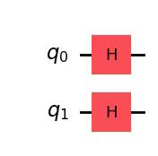
We can create a two-qubit quantum circuit with following code. We will apply an H gate to each qubit.
# Create the two qubits quantum circuit
qc = QuantumCircuit(2)

# Apply an H gate to qubit 0
qc.h(0)

# Apply an H gate to qubit 1
qc.h(1)

# Draw the circuit
qc.draw(output="mpl")
Output:
# See the statevector
out_vector = Statevector(qc)
print(out_vector)
Output:
Statevector([0.5+0.j, 0.5+0.j, 0.5+0.j, 0.5+0.j],
            dims=(2, 2))
Note: Qiskit bit ordering
Qiskit uses Little Endian notation when ordering qubits and bits, meaning qubit 0 is the rightmost bit in the bitstrings. Example: means q0 is and q1 is . Be careful because some literature in quantum computing use the Big Endian notation (qubit 0 is the leftmost bit) and a great deal of quantum mechanics literature does, too.
Another thing to notice is that when representing a quantum circuit, is always placed at the top of the circuit.
With this in mind, the quantum state of the above circuit can be written as a tensor product of single-qubit quantum state.
( )
The initial state of Qiskit is , so by applying to each qubit, it changes to a state of equal superposition.
The measurement rule is also same as a single qubit case, the probability of measuring is .
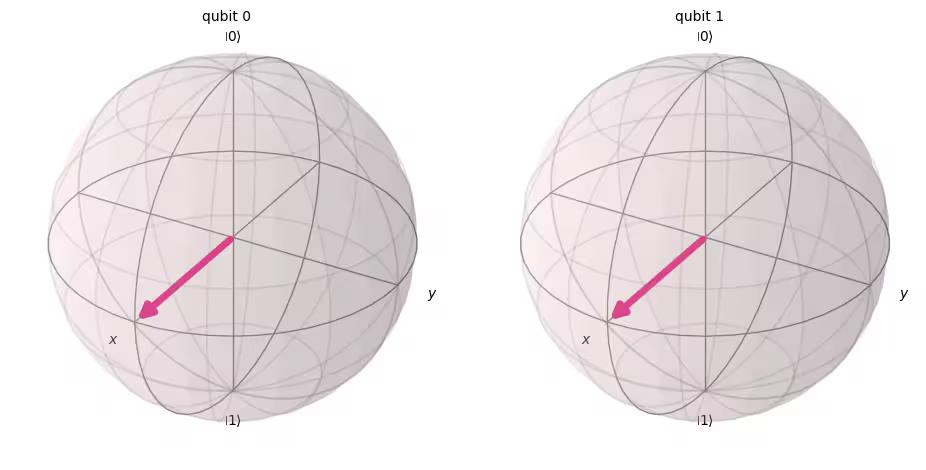
# Draw a Bloch sphere
plot_bloch_multivector(out_vector)
Output:
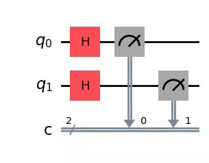
Next, let's measure this circuit.
# Create a new circuit with two qubits (first argument) and two classical bits (second argument)
qc = QuantumCircuit(2, 2)

# Apply the gates
qc.h(0)
qc.h(1)

# Add the measurement gates
qc.measure(0, 0)  # Measure qubit 0 and save the result in bit 0
qc.measure(1, 1)  # Measure qubit 1 and save the result in bit 1

# Draw the circuit
qc.draw(output="mpl")
Output:
Now, we will use a Aer simulator, again, to experimentally verify that the relative probabilities of all possible output states are roughly equal.
# Run the circuit on a simulator to get the results
# Define backend
backend = AerSimulator()
# Transpile to backend
pm = generate_preset_pass_manager(backend=backend, optimization_level=1)
isa_qc = pm.run(qc)
# Run the job
sampler = Sampler(mode=backend)
job = sampler.run([isa_qc])
result = job.result()
# Print the results
counts = result[0].data.c.get_counts()
print(counts)
# Plot the counts in a histogram
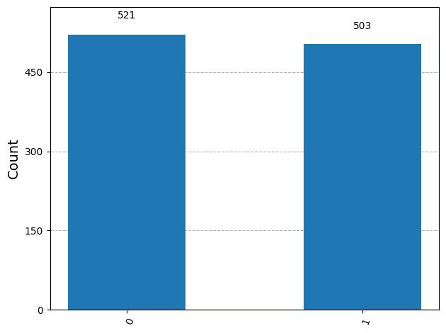
plot_histogram(counts)Output:
{'10': 262, '01': 246, '00': 265, '11': 251}
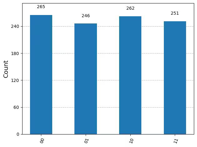
As expected, the states , , , were measured almost 25% each.
4.2 Multi-qubit quantum gates
CNOT gate
A CNOT("controlled NOT" or CX) gate is a two-qubit gate, meaning its action involves two qubits at once: the control qubit and the target qubit. A CNOT flips the target qubit only when the control qubit is .
Input (target,control) | Output (target,control) |
|---|---|
| 00 | 00 |
| 01 | 11 |
| 10 | 10 |
| 11 | 01 |
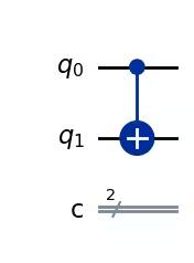
Let us first simulate the action of this two-qubit gate when q0 and q1 are both , and obtain the output statevector. The Qiskit syntax used is qc.cx(control qubit, target qubit).
# Create a circuit with two quantum registers and two classical registers
qc = QuantumCircuit(2, 2)

# Apply the CNOT (cx) gate to a |00> state.
qc.cx(0, 1)  # Here the control is set to q0 and the target is set to q1.

# Draw the circuit
qc.draw(output="mpl")
Output:
# See the statevector
out_vector = Statevector(qc)
print(out_vector)
Output:
Statevector([1.+0.j, 0.+0.j, 0.+0.j, 0.+0.j],
            dims=(2, 2))
As expected, applying a CNOT gate on did not change the state, since the control qubit was in the state.
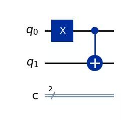
Let's get back to our CNOT operation. This time we will apply a CNOT gate to and see what happens.
qc = QuantumCircuit(2, 2)

# q0=1, q1=0
qc.x(0)  # Apply a X gate to initialize q0 to 1
qc.cx(0, 1)  # Set the control bit to q0 and the target bit to q1.

# Draw the circuit
qc.draw(output="mpl")
Output:
# See the statevector
out_vector = Statevector(qc)
print(out_vector)
Output:
Statevector([0.+0.j, 0.+0.j, 0.+0.j, 1.+0.j],
            dims=(2, 2))
By applying a CNOT gate, the state has now become .
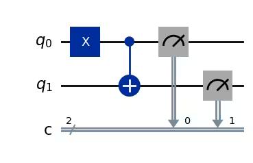
Let us verify these results by running the circuit on a simulator.
# Add measurements
qc.measure(0, 0)
qc.measure(1, 1)

# Draw the circuit
qc.draw(output="mpl")
Output:
# Run the circuit on a simulator to get the results
# Define backend
backend = AerSimulator()

# Transpile to backend
pm = generate_preset_pass_manager(backend=backend, optimization_level=1)
isa_qc = pm.run(qc)

# Run the job
sampler = Sampler(backend)
job = sampler.run([isa_qc])
result = job.result()

# Print the results
counts = result[0].data.c.get_counts()
print(counts)

# Plot the counts in a histogram
plot_histogram(counts)
Output:
{'11': 1024}
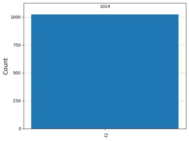
The results should show you that has been measured with 100% probability.
4.3 Quantum entanglement and execution on a real quantum device
Let's start by introducing a specific entangled state which is particularly important in quantum computation, then we'll define the term "entangled":
and this state is called a Bell state.
An entangled state is a state consisting of quantum states and that cannot be represented by a tensor product of individual quantum states.
If below has two states and ;
the tensor product of these two states is the following
but there are no coefficients and to satisfy these two equations. Therefore, is not represented by a tensor product of individual quantum state, and , and this means that is entangled state.
Let us create the Bell state and run it on a real quantum computer. Now we will follow the four steps to writing a quantum program, called Qiskit patterns:
- Map problem to quantum circuits and operators
- Optimize for target hardware
- Execute on target hardware
- Post-process the results
Step 1. Map problem to quantum circuits and operators
In a quantum program, quantum circuits are the native format in which to represent quantum instructions. When creating a circuit, you'll usually create a new QuantumCircuit object, then add instructions to it in sequence.
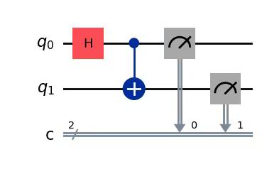
The following code cell creates a circuit that produces a Bell state, the specific two-qubit entangled state from above.
qc = QuantumCircuit(2, 2)

qc.h(0)
qc.cx(0, 1)

qc.measure(0, 0)
qc.measure(1, 1)

qc.draw("mpl")
Output:
Step 2. Optimize for target hardware
Qiskit converts abstract circuits to QISA (Quantum Instruction Set Architecture) circuits that respect the constraints of the target hardware and optimizes circuit performance. So before the optimization, we will specify the target hardware.
If you do not have qiskit-ibm-runtime, you will need to install this first. For more information about Qiskit Runtime, check out the API reference.
# Install
# !pip install qiskit-ibm-runtime
We will specify the target hardware.
from qiskit_ibm_runtime import QiskitRuntimeService

service = QiskitRuntimeService()
service.backends()
# You can specify the device
# backend = service.backend('ibm_kingston')# You can also identify the least busy device
backend = service.least_busy(operational=True)
print("The least busy device is ", backend)Transpiling the circuit is yet another complex process. Very briefly, this rewrites the circuit into a logically equivalent one using "native gates" (gates that a particular quantum computer can implement) and maps the qubits in your circuit to optimal real qubits on the target quantum computer. For more on transpilation, see this documentation.
# Transpile the circuit into basis gates executable on the hardware
pm = generate_preset_pass_manager(backend=backend, optimization_level=1)
target_circuit = pm.run(qc)

target_circuit.draw("mpl", idle_wires=False)
You can see that in the transpilation the circuit was rewritten using new gates. For more information, refer to the ECRGate documentation.
Step 3. Execute the target circuit
Now, we will run the target circuit on the real device.
sampler = Sampler(backend)
job_real = sampler.run([target_circuit])

job_id = job_real.job_id()
print("job id:", job_id)
Execution on the real device might require waiting in a queue, since quantum computers are valuable resources, and very much in demand. The job_id is used to check the execution status and results of the job later.
# Check the job status (replace the job id below with your own)
job_real.status(job_id)
You can also check the job status from your IBM Quantum dashboard:https://quantum.cloud.ibm.com/workloads
# If the Notebook session got disconnected you can also check your job status
# by running the following code
from qiskit_ibm_runtime import QiskitRuntimeService

service = QiskitRuntimeService()
job_real = service.job(job_id)  # Input your job-id between the quotations
job_real.status()
# Execute after job has successfully run
result_real = job_real.result()
print(result_real[0].data.c.get_counts())Step 4. Post-process the results
Finally, we must post-process our results to create outputs in the expected format, like values or graphs.
plot_histogram(result_real[0].data.c.get_counts())As you can see, and are the most frequently observed. There are a few results other than the expected data, and they are due to noise and qubit decoherence. We will learn more about errors and noise in quantum computers in the later lessons of this course.
4.4 GHZ state
The concept of entanglement can be extended to systems of more than two qubits. The GHZ state (Greenberger-Horne-Zeilinger state) is a maximally entangled state of three or more qubits. The GHZ state for three qubits is defined as
It can be created with the following quantum circuit.
qc = QuantumCircuit(3, 3)

qc.h(0)
qc.cx(0, 1)
qc.cx(1, 2)

qc.measure(0, 0)
qc.measure(1, 1)
qc.measure(2, 2)

qc.draw("mpl")
Output:
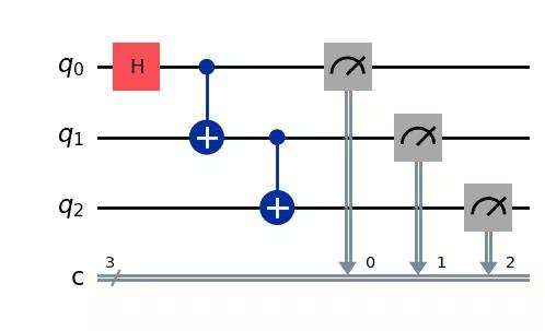
The "depth" of a quantum circuit is a useful and common metric to describe quantum circuits. Trace a path through the quantum circuit, moving left to right, only changing qubits when they are connected by a multi-qubit gate. Count the number of gates along that path. The maximum number of gates for any such path through a circuit is the depth. In modern noisy quantum computers, low-depth circuits have fewer errors and are likely to return good results. Very deep circuits are not.
Using QuantumCircuit.depth(), we can check the depth of our quantum circuit. The depth of the above circuit is 4. The top qubit has only three gates including the measurement. But there is a path from the top qubit down to either qubit 1 or qubit 2 which involves another CNOT gate.
qc.depth()Output:
4
Exercise 2
The GHZ state of an 8-qubit system is
Write code to prepare this state with the shallowest possible circuit. The depth of the shallowest quantum circuit is 5, including the measurement gates.
Solution:
# Step 1
qc = QuantumCircuit(8, 8)

##your code goes here##
qc.h(0)
qc.cx(0, 4)
qc.cx(4, 6)
qc.cx(6, 7)

qc.cx(4, 5)

qc.cx(0, 2)
qc.cx(2, 3)

qc.cx(0, 1)
qc.barrier()  # for visual separation

# measure
for i in range(8):
    qc.measure(i, i)

qc.draw("mpl")
# print(qc.depth())
Output:
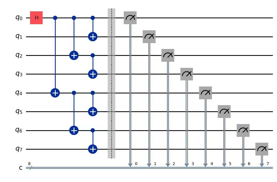
print(qc.depth())Output:
5
from qiskit.visualization import plot_histogram
# Step 2
# For this exercise, the circuit and operators are simple, so no optimizations are needed.
# Step 3
# Run the circuit on a simulator to get the results
backend = AerSimulator()
pm = generate_preset_pass_manager(backend=backend, optimization_level=1)
isa_qc = pm.run(qc)
sampler = Sampler(mode=backend)
job = sampler.run([isa_qc], shots=1024)
result = job.result()
counts = result[0].data.c.get_counts()
print(counts)
# Step 4
# Plot the counts in a histogram
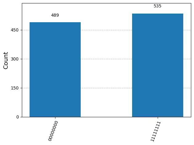
plot_histogram(counts)Output:
{'11111111': 535, '00000000': 489}
5. Summary
You have learned quantum computation with the circuit model using quantum bits and gates, and you have reviewed superposition, measurement, and entanglement. You also have learned the method to execute the quantum circuit on the real quantum device.
In the final exercise to create a GHZ circuit, you have tried to reduce the circuit depth, which is an important factor for obtaining a utility scale solution in a noisy quantum computer. In the later lessons of this course, you will learn about noise and about error mitigation methods in detail. In this lesson, as an introduction, we considered reducing the circuit depth in an ideal device, but in reality, we must consider the constraints of real device, such as qubit connectivity. You will learn more about this in subsequent lessons in this course.
# See the version of Qiskit
import qiskit

qiskit.__version__
Output:
'2.0.2'