Quantum algorithms: Phase estimation
Kento Ueda (15 May 2024)
This notebook provides the fundamental concepts and implementation of the Quantum Fourier Transformation (QFT) and Quantum Phase Estimation (QPE).
Download the pdf of the original lecture. Note that some code snippets might become deprecated since these are static images.
Approximate QPU time to run this experiment is 7 seconds.
1. Introduction
Quantum Fourier Transformation (QFT)
The Quantum Fourier Transformation is the quantum counterpart of the classical discrete Fourier transform. It is a linear transformation applied to the quantum states, mapping computational bases into their Fourier basis representations. The QFT plays a key role in many quantum algorithms, offering an efficient method to extract periodicity information from quantum states. The QFT can be implemented with operations with quantum gates such as Hadamard gates and Control-Phase gates for qubits, enabling exponential speedup over classical Fourier transformation.
- Applications: It is a foundational part in quantum algorithms such as Shor's algorithm for factoring large integers and discrete logarithm.
Quantum Phase Estimation (QPE)
Quantum Phase Estimation is a quantum algorithm used to estimate the phase associated with an eigenvector of a unitary operator. This algorithm provides a bridge between the abstract mathematical properties of quantum states and their computational applications.
- Applications: It can solve problems such as finding eigenvalues of unitary matrices and simulating quantum systems.
Together, QFT and QPE form the essential backbone of many quantum algorithms solving problems that are infeasible for classical computers. By the end of this notebook, you will gain an understanding of how these techniques are implemented.
2. Basic of Quantum Fourier Transformation (QFT)
from qiskit import QuantumCircuit, QuantumRegister, ClassicalRegister
from qiskit_aer import AerSimulator
from qiskit.visualization import plot_histogram, plot_bloch_multivector
from qiskit.quantum_info import Statevector
from qiskit.transpiler.preset_passmanagers import generate_preset_pass_manager
from qiskit_ibm_runtime import Sampler

from numpy import pi
From the analogy with the discrete Fourier transform, the QFT acts on a quantum state for qubits and maps it to the quantum state .
where .
Or the unitary matrix representation:
2.1. Intuition
The quantum Fourier transform (QFT) transforms between two bases, the computational (Z) basis, and the Fourier basis. But what does the Fourier basis mean in this context? You likely recall that the Fourier transform of a function describes the convolution of onto a sinusoidal function with frequency . In Layman's terms: the Fourier transform is a function describing how much of each frequency we would need to build up a function out of sine functions (or cosine functions). To get a better sense for what the QFT means in this context, consider the stepped images below which show a number encoded in binary, using four qubits:
In the computational basis, we store numbers in binary using the states and .
Note the frequency with which the different qubits change; the leftmost qubit flips with every increment in the number, the next with every 2 increments, the third with every 4 increments, and so on.
If we apply a quantum Fourier transform to these states, we map
(We often denote states in the Fourier basis using the tilde (~)).
In the Fourier basis, we store numbers using different rotations around the Z-axis:
IFRAME
The number we want to store dictates the angle at which each qubit is rotated around the Z-axis. In the state , all qubits are in the state . As seen in the example above, to encode the state on 4 qubits, we rotated the leftmost qubit by full turns ( radians). The next qubit is turned double this ( radians, or full turns), this angle is then doubled for the qubit after, and so on.
Again, note the frequency with which each qubit changes. The leftmost qubit (qubit 0) in this case has the lowest frequency, and the rightmost the highest.
2.2 Example: 1-qubit QFT
Let's consider the case of .
The unitary matrix can be written:
This operation is the result of applying the Hadamard gate ().
2.3 Product representation of QFT
Let's generalize a transformation for , acting on the state .
2.4 Example: Circuit construction of 3 qubits QFT
From the above description, it might not be clear how to construct a QFT circuit. For now, simply note that we expect three qubits to have phases that evolve at different "rates". Understand exactly how this is translated into a circuit is left as an exercise to the reader. There are multiple diagrams and examples in the lecture pdf. Additional resources include this lesson from the Fundamentals of quantum algorithms course.
We will demonstrate QFT using simulators only, and thus we will not use the Qiskit patterns framework until we move on to quantum phase estimation.
# Prepare for 3 qubits circuit
qr = QuantumRegister(3)
cr = ClassicalRegister(3)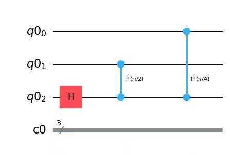
qc = QuantumCircuit(qr, cr)qc.h(2)
qc.cp(pi / 2, 1, 2) # Controlled-phase gate from qubit 1 to qubit 2
qc.cp(pi / 4, 0, 2) # Controlled-phase gate from qubit 0 to qubit 2
qc.draw(output="mpl")Output:
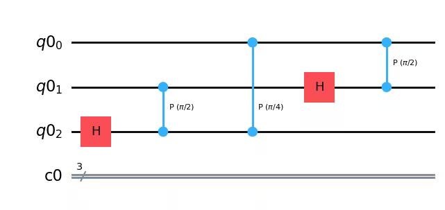
qc.h(1)
qc.cp(pi / 2, 0, 1)  # Controlled-phase gate from qubit 0 to qubit 1

qc.draw(output="mpl")
Output:
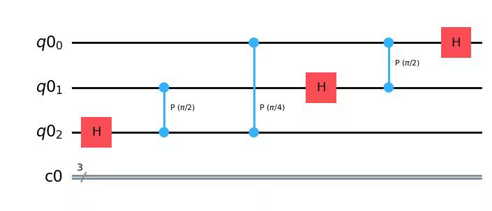
qc.h(0)

qc.draw(output="mpl")
Output:
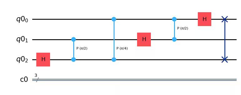
qc.swap(0, 2)

qc.draw(output="mpl")
Output:
We try to apply QFT to as an example.
First, we confirm the binary notation of the integer 5 and create the circuit encoding the state 5:
bin(5)Output:
'0b101'
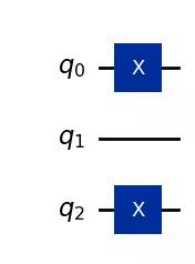
qc = QuantumCircuit(3)

qc.x(0)
qc.x(2)
qc.draw(output="mpl")
Output:
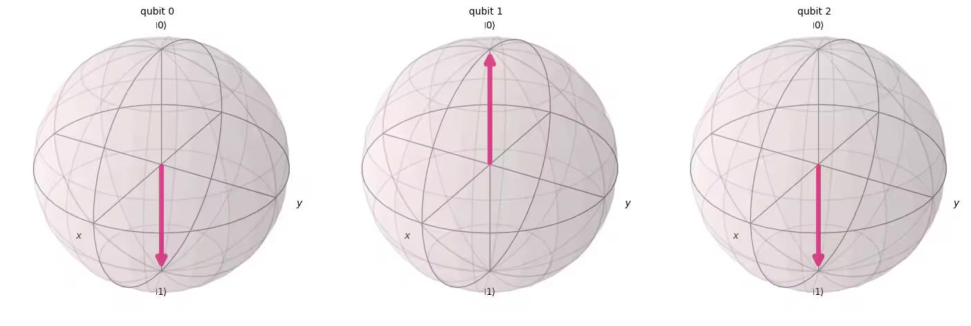
We check the quantum states using the Aer simulator:
statevector = Statevector(qc)
plot_bloch_multivector(statevector)
Output:
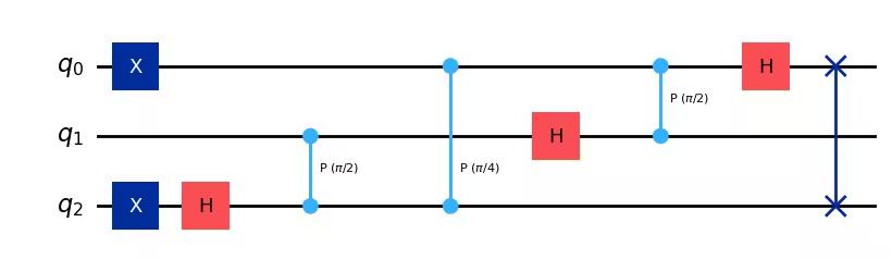
Finally, we add QFT and view the final state of our qubits:
qc.h(2)
qc.cp(pi / 2, 1, 2)
qc.cp(pi / 4, 0, 2)

qc.h(1)
qc.cp(pi / 2, 0, 1)

qc.h(0)

qc.swap(0, 2)

qc.draw(output="mpl")
Output:
statevector = Statevector(qc)
plot_bloch_multivector(statevector)
Output:
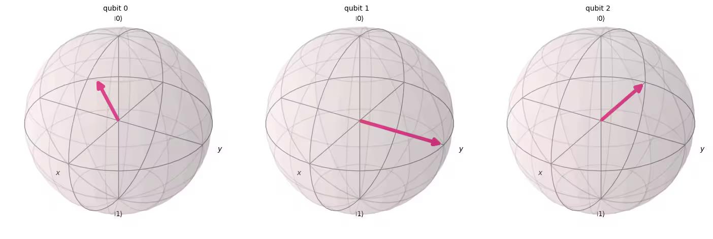
We can see out QFT function has worked correctly. Qubit 0 has been rotated by of a full turn, qubit 1 by full turns (equivalent to of a full turn), and qubit 2 by full turns (equivalent to of a full turn).
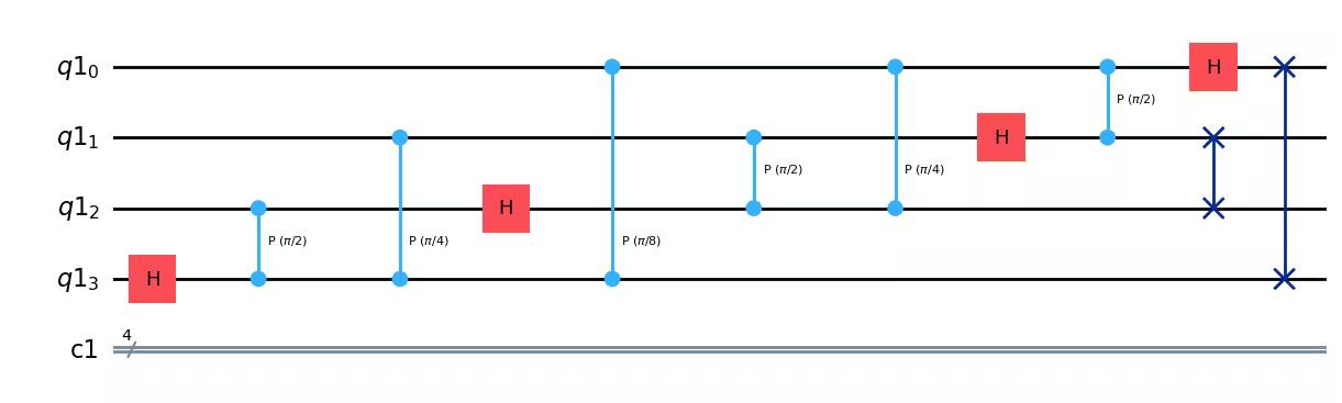
2.5 Exercise: QFT
(1) Implement QFT of 4 qubits.
##your code goes here##(2) Apply QFT to , simulate and plot the statevector using the Bloch sphere.
##your code goes here##Solution of the exercise: QFT
(1)
qr = QuantumRegister(4)
cr = ClassicalRegister(4)
qc = QuantumCircuit(qr, cr)

qc.h(3)
qc.cp(pi / 2, 2, 3)
qc.cp(pi / 4, 1, 3)
qc.cp(pi / 8, 0, 3)

qc.h(2)
qc.cp(pi / 2, 1, 2)
qc.cp(pi / 4, 0, 2)

qc.h(1)
qc.cp(pi / 2, 0, 1)

qc.h(0)

qc.swap(0, 3)
qc.swap(1, 2)

qc.draw(output="mpl")
Output:
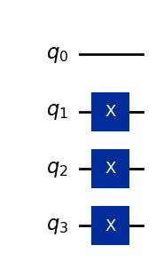
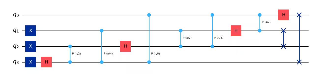
(2)
bin(14)Output:
'0b1110'
qc = QuantumCircuit(4)

qc.x(1)
qc.x(2)
qc.x(3)
qc.draw("mpl")
Output:
qc.h(3)
qc.cp(pi / 2, 2, 3)
qc.cp(pi / 4, 1, 3)
qc.cp(pi / 8, 0, 3)

qc.h(2)
qc.cp(pi / 2, 1, 2)
qc.cp(pi / 4, 0, 2)

qc.h(1)
qc.cp(pi / 2, 0, 1)
qc.h(0)

qc.swap(0, 3)
qc.swap(1, 2)

qc.draw(output="mpl")
Output:
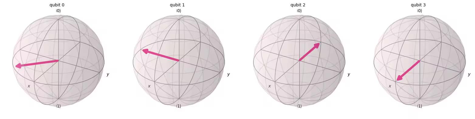
statevector = Statevector(qc)
plot_bloch_multivector(statevector)
Output:
3. Basics of Quantum Phase Estimation (QPE)
Given a unitary operation , the QPE estimates in since is unitary, all of its eigenvalues have a norm of 1.
3.1 Procedure
1. Setup
is in one set of qubit registers. An additional set of qubits form the counting register on which we will store the value :
2. Superposition
Apply a -bit Hadamard gate operation on the counting register:
3. Controlled Unitary operations
We need to introduce the controlled unitary that applies the unitary operator on the target register only if its corresponding control bit is . Since is a unitary operator with eigenvector such that , this means:
3.2 Example: T-gate QPE
Let's use gate as an example of QPE and estimate its phase .
We expect to find:
where
We initialize of the eigenvector of gate by applying an gate:
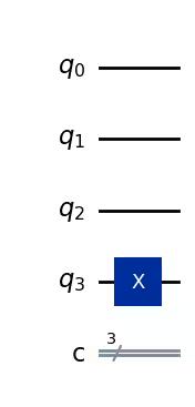
qpe = QuantumCircuit(4, 3)
qpe.x(3)
qpe.draw(output="mpl")
Output:
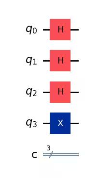
Next, we apply Hadamard gates to the counting qubits:
for qubit in range(3):
    qpe.h(qubit)
qpe.draw(output="mpl")
Output:
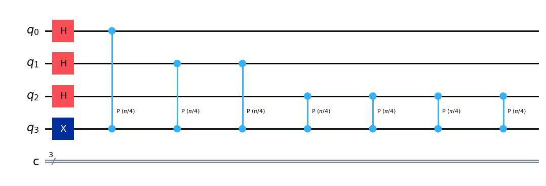
We perform the controlled unitary operations:
repetitions = 1
for counting_qubit in range(3):
    for i in range(repetitions):
        qpe.cp(pi / 4, counting_qubit, 3)  # This is C-U
    repetitions *= 2
qpe.draw(output="mpl")
Output:
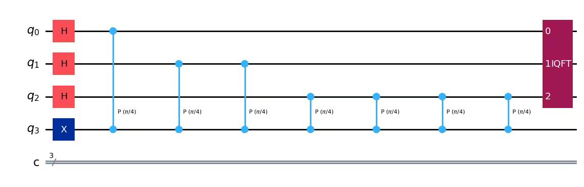
We apply the inverse quantum Fourier transformation to convert the state of the counting register, then measure the counting register:
from qiskit.circuit.library import QFT# Apply inverse QFT
qpe.append(QFT(3, inverse=True), [0, 1, 2])
qpe.draw(output="mpl")Output:
for n in range(3):
    qpe.measure(n, n)
qpe.draw(output="mpl")
Output:
We can simulate using Aer simulator:
aer_sim = AerSimulator()
shots = 2048

pm = generate_preset_pass_manager(backend=aer_sim, optimization_level=1)
t_qpe = pm.run(qpe)

sampler = Sampler(mode=aer_sim)
job = sampler.run([t_qpe], shots=shots)
result = job.result()
answer = result[0].data.c.get_counts()

plot_histogram(answer)
Output:
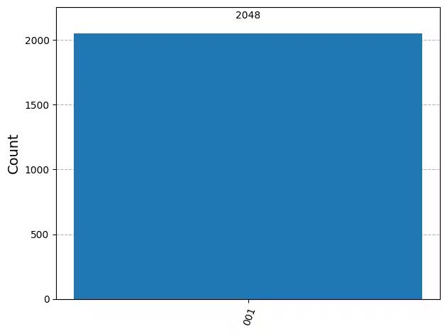
We see we get one result (001) with certainty, which translates to the decimal: 1. We now need to divide our result (1) by to get :
Shor's algorithm allows us to factorize a number by building a circuit with unknown and obtaining .
3.3 Exercise
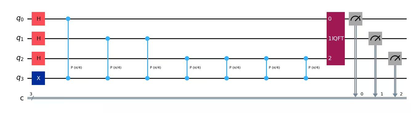
Estimate using 3 qubits for counting and a qubit for an eigenvector.
. Since we want to implement , we need to set .
##your code goes here##Solution of the exercise:
# Create and set up circuit
qpe = QuantumCircuit(4, 3)

# Apply H-Gates to counting qubits:
for qubit in range(3):
    qpe.h(qubit)

# Prepare our eigenstate |psi>:
qpe.x(3)

# Do the controlled-U operations:
angle = 2 * pi / 3
repetitions = 1
for counting_qubit in range(3):
    for i in range(repetitions):
        qpe.cp(angle, counting_qubit, 3)
    repetitions *= 2

# Do the inverse QFT:
qpe.append(QFT(3, inverse=True), [0, 1, 2])

for n in range(3):
    qpe.measure(n, n)

qpe.draw(output="mpl")
Output:

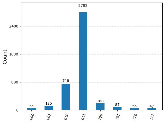
aer_sim = AerSimulator()
shots = 4096

pm = generate_preset_pass_manager(backend=aer_sim, optimization_level=1)
t_qpe = pm.run(qpe)

sampler = Sampler(mode=aer_sim)
job = sampler.run([t_qpe], shots=shots)
result = job.result()
answer = result[0].data.c.get_counts()

plot_histogram(answer)
Output:
4. Execution using the Qiskit Runtime Sampler primitive
We will perform QPE using the real quantum device and follow 4 steps of Qiskit patterns.
- Map the problem to a quantum-native format
- Optimize the circuits
- Execute the target circuit
- Post-process the results
from qiskit_ibm_runtime import QiskitRuntimeService
from qiskit_ibm_runtime import Sampler
# Loading your IBM Quantum® account(s)
service = QiskitRuntimeService()4.1 Step 1: Map problem to quantum circuits and operators
qpe = QuantumCircuit(4, 3)
qpe.x(3)
for qubit in range(3):
    qpe.h(qubit)
repetitions = 1
for counting_qubit in range(3):
    for i in range(repetitions):
        qpe.cp(pi / 4, counting_qubit, 3)  # This is C-U
    repetitions *= 2
qpe.append(QFT(3, inverse=True), [0, 1, 2])
for n in range(3):
    qpe.measure(n, n)
qpe.draw(output="mpl")
Output:

backend = service.least_busy(simulator=False, operational=True, min_num_qubits=4)

print(backend)
Output:
<IBMBackend('ibm_strasbourg')>
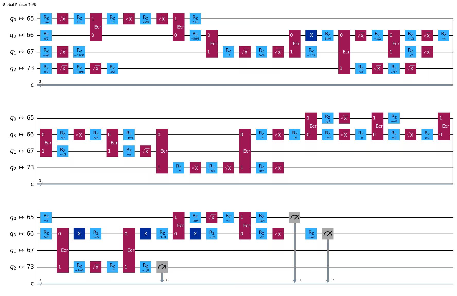
4.2 Step 2: Optimize for target hardware
# Transpile the circuit into basis gates executable on the hardware
pm = generate_preset_pass_manager(backend=backend, optimization_level=2)
qc_compiled = pm.run(qpe)

qc_compiled.draw("mpl", idle_wires=False)
Output:
4.3 Step 3: Execute on target hardware
real_sampler = Sampler(mode=backend)
job = real_sampler.run([qc_compiled], shots=1024)
job_id = job.job_id()
print("job id:", job_id)
Output:
job id: d13p4zb5z6q00087ag00
job = service.job(job_id)  # Input your job-id between the quotations
job.status()
Output:
'DONE'
result_real = job.result()
print(result_real)
Output:
PrimitiveResult([SamplerPubResult(data=DataBin(c=BitArray(<shape=(), num_shots=1024, num_bits=3>)), metadata={'circuit_metadata': {}})], metadata={'execution': {'execution_spans': ExecutionSpans([DoubleSliceSpan(<start='2025-06-09 22:39:00', stop='2025-06-09 22:39:00', size=1024>)])}, 'version': 2})
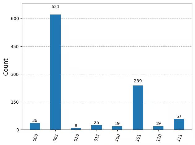
4.4 Step 4: Post-process the results
from qiskit.visualization import plot_histogram

plot_histogram(result_real[0].data.c.get_counts())
Output:
# See the version of Qiskit
import qiskit

qiskit.__version__
Output:
'2.0.2'