量子近似最適化アルゴリズム
使用時間の見積もり:Heron r3 プロセッサーで22分(注:これはあくまでも見積もりです。 ランタイムは異なるかもしれない)。
学習成果
- 古典的な組み合わせ最適化問題(最大カット問題)を量子ハミルトニアンに写像する方法
- IBM Quantum Compute Service セッションを使用して、量子近似最適化アルゴリズム(QAOA)を実装および実行する方法
- 小規模なシミュレータ例から実用規模のハードウェア実行へとQAOAワークフローを拡張する方法
前提条件
背景
量子近似最適化アルゴリズム(QAOA) は、組み合わせ最適化問題を解くための、量子と古典を組み合わせた反復法である。 このチュートリアルでは、QAOAを用いて最大カット(max-cut) 問題を解きます。これは、クラスタリング、ネットワーク科学、統計物理学などの分野で応用されるNP困難な最適化問題です。 辺で結ばれたノードからなるグラフに対し、分割線を横切る辺の数が最大になるように、ノードを2つの集合に分割することを目的とする。
組み合わせ最適化は、燃料消費を削減するための配送ルートの計画や、資材の無駄を最小限に抑えるための資源配分など、持続可能性に関する課題においても活用されています。 max-cutの例では、目的関数をコストハミルトニアンとして表現し、QAOAを用いて解の候補を探索するプロセスについて解説します。 このアプローチを持続可能性の問題に適用するには、その適用目的を反映した目的関数と制約条件が必要となる。
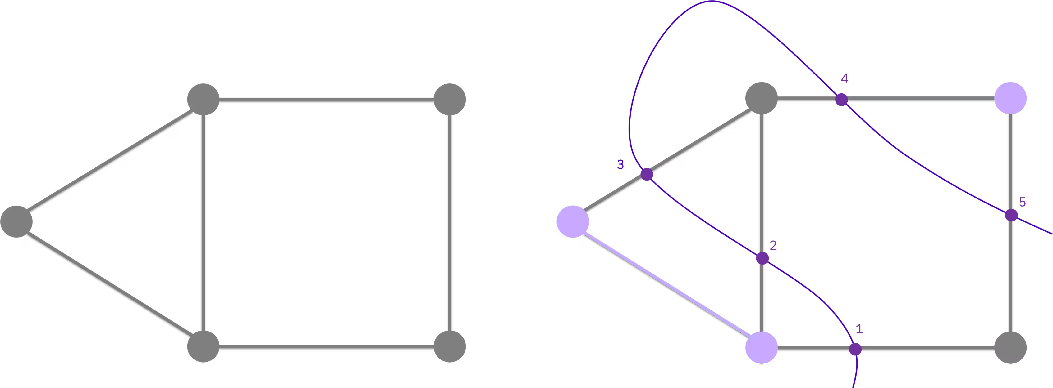
古典的最適化から量子回路へ
Max-cutは、古典的な二値最適化問題として定式化することができる。 各ノードには、どの集合に属するかを示す二値変数 が割り当てられる。 目的は、端点が異なる集合に属する辺の数を最大化することです:
これは、 という形式の二次制約なし二値最適化(QUBO) 問題に相当する。標準的な変数置換( )を用いることで、このQUBOはコストハミルトニアンとして書き換えることができ、その基底状態が最適解を符号化する。 一般に、このハミルトニアンには二次項と一次項の両方が含まれている:
ここで検討する非加重最大切断問題では、各辺について線形係数はゼロ( )となり、 となるため、以下のコードで実装するより単純な形 が得られます。 上記のより一般的な形式は、このワークフローを重み付きグラフやその他のQUBOで表現可能な問題に適用する際に必要となるものです。
QAOAの仕組み
QAOAは、初期の重ね合わせ状態 に対して、 コスト演算子 とミキサー演算子 の2つの演算子を交互に重ね合わせて、候補解を生成する。角度 および は、古典的なフィードバックループで最適化される。量子コンピュータがコスト関数を評価し、古典的な最適化アルゴリズムが収束するまでパラメータを更新する。 この反復ループは、Quantum Compute セッション内で実行されます。これにより、反復処理の間、量子デバイスが予約された状態が維持され、レイテンシの低減が図られます。
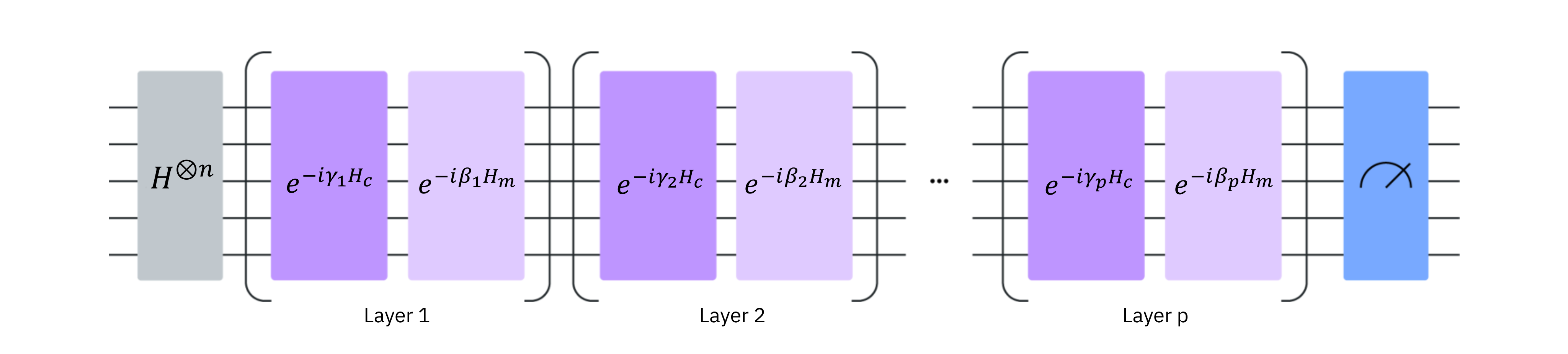
QUBOからハミルトニアンへの完全な導出を含む、QAOA理論に関するより詳細な解説については、 QAOAコースのモジュールをご覧ください。
このチュートリアルでは、まず5ノードの小さなグラフで最大切断問題を解き、その後、実際のハードウェア上で、同じワークフローを100ノードのユーティリティ規模の問題に拡張します。 プランの利用に関する注意事項: このチュートリアルでは「Quantum Compute」 セッションを使用していますが、これは「プレミアムプラン」でのみ利用可能です。 「Open Plan」プランをご利用の場合は、このチュートリアルを記載通りに実行することはできません。代わりに、をジョブモード Session に切り替える必要があります(つまり、最適化ループをで囲むのではなく、各反復を独立したジョブとして送信します Session(...))。 ワークフローは引き続き実行されますが、各反復処理において、予約済みのデバイスを再利用するのではなく、キューのレイテンシを全額負担することになります。 詳細については、「 利用可能なプランの概要」 をご覧ください。
要件
このチュートリアルを始める前に、以下のものがインストールされていることを確認してください:
- Qiskit SDK v2.0 以降、 可視化機能を搭載
- Qiskit Runtime v0.22 またはそれ以降 (
pip install qiskit-ibm-runtime)
また、 IBM Quantum® Platform 上のインスタンスにアクセスできる必要があります。
セットアップ
import matplotlib.pyplot as plt
import rustworkx as rx
from rustworkx.visualization import mpl_draw as draw_graph
import numpy as np
from scipy.optimize import minimize
from collections import defaultdict
from typing import Sequence


from qiskit.quantum_info import SparsePauliOp
from qiskit.circuit.library import QAOAAnsatz
from qiskit.transpiler.preset_passmanagers import generate_preset_pass_manager

from qiskit_ibm_runtime import QiskitRuntimeService
from qiskit_ibm_runtime import Session, EstimatorV2 as Estimator
from qiskit_ibm_runtime import SamplerV2 as Sampler
小規模な例
このセクションでは、5ノードの小さな最大切断問題のインスタンスを用いて、QAOAワークフローの各ステップを順を追って説明します。 「小規模」と銘打たれてはいるものの、この例は実際の IBM Quantum ハードウェア上で動作します。コードは127キュービット以上のバックエンドを選択し、そこで回路を実行します。
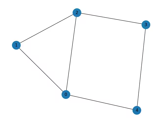
のノードでグラフを作成し、問題を初期化する。
n_small = 5

graph = rx.PyGraph()
graph.add_nodes_from(np.arange(0, n_small, 1))
edge_list = [
    (0, 1, 1.0),
    (0, 2, 1.0),
    (0, 4, 1.0),
    (1, 2, 1.0),
    (2, 3, 1.0),
    (3, 4, 1.0),
]
graph.add_edges_from(edge_list)
draw_graph(graph, node_size=600, with_labels=True)
Output:
ステップ1:古典的な入力を量子問題にマッピングする
古典グラフを量子回路および演算子に写像する。 「 背景 」で述べたように、重みなし最大切断問題において、コストハミルトニアンは に還元され、QAOAではパラメータ化されたアンザッツ回路を用いて、 という候補基底状態を生成する。
コストハミルトニアンを構築する
グラフの辺をパウリ 項に変換し、 を構築する(導出については 「背景」 を参照)。
def build_max_cut_paulis(
    graph: rx.PyGraph,
) -> list[tuple[str, list[int], float]]:
    """Convert graph edges to a list of ZZ Pauli terms.

    The returned list is in the sparse format expected by
    ``SparsePauliOp.from_sparse_list``: each element is
    ``(pauli_string, qubit_indices, coefficient)``.
    """
    pauli_list = []
    for edge in list(graph.edge_list()):
        weight = graph.get_edge_data(edge[0], edge[1])
        pauli_list.append(("ZZ", [edge[0], edge[1]], weight))
    return pauli_list


max_cut_paulis = build_max_cut_paulis(graph)
cost_hamiltonian = SparsePauliOp.from_sparse_list(max_cut_paulis, n_small)
print("Cost Function Hamiltonian:", cost_hamiltonian)
Output:
Cost Function Hamiltonian: SparsePauliOp(['IIIZZ', 'IIZIZ', 'ZIIIZ', 'IIZZI', 'IZZII', 'ZZIII'],
              coeffs=[1.+0.j, 1.+0.j, 1.+0.j, 1.+0.j, 1.+0.j, 1.+0.j])
QAOAアンザッツ回路を構築する
を使用して QAOAAnsatz 、コストハミルトニアンからパラメータ化されたQAOA回路を構築する。 ここでは、(2つのQAOA層、4つのパラメータ: )を使用 reps=2 する。
circuit = QAOAAnsatz(cost_operator=cost_hamiltonian, reps=2)
circuit.measure_all()

circuit.draw("mpl")
Output:

circuit.parametersOutput:
ParameterView([ParameterVectorElement(β[0]), ParameterVectorElement(β[1]), ParameterVectorElement(γ[0]), ParameterVectorElement(γ[1])])
ステップ2:量子ハードウェア実行に向けた問題の最適化
抽象回路をハードウェア固有の命令に変換する。 このステップでは、量子ビットのマッピング、ゲートの分解、ルーティング、およびエラー抑制を行います。 詳細については、トランスパイルに関するドキュメントを参照してください。
service = QiskitRuntimeService()
backend = service.least_busy(
    operational=True, simulator=False, min_num_qubits=127
)
print(backend)

# Create pass manager for transpilation. Level 3 is the most aggressive
# preset: slower to transpile, but produces shorter circuits that are
# more robust to hardware noise.
pm = generate_preset_pass_manager(optimization_level=3, backend=backend)

candidate_circuit = pm.run(circuit)
candidate_circuit.draw("mpl", fold=False, idle_wires=False)
Output:
<IBMBackend('ibm_pittsburgh')>

ステップ3: Qiskit primitivesを使用して実行する
QAOAの最適化ループは、反復処理の間、デバイスが確保された状態を維持するために、Quantum Compute セッション内で実行されます。 推定器は各ステップで を評価し、従来の最適化アルゴリズム(COBYLA)は収束するまでパラメータを更新します。
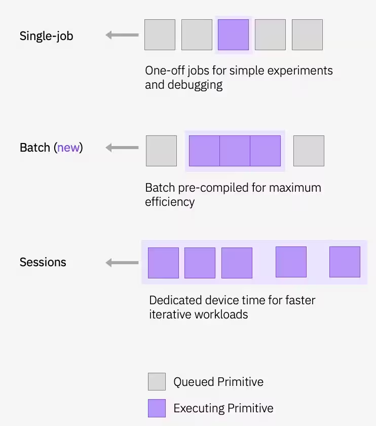
初期パラメータを定義し、最適化ループを実行します:
# QAOA doesn't prescribe principled default angles — any bounded choice
# works as a warm start for problems this small. beta and gamma are
# periodic (beta in [0, pi] and gamma in [0, 2*pi] modulo the underlying
# Pauli-rotation periods), and pi/2 and pi are just midpoints of those
# ranges. For harder problems you would typically warm start from known
# good angles or transfer parameters from smaller instances.
initial_gamma = np.pi
initial_beta = np.pi / 2
init_params = [initial_beta, initial_beta, initial_gamma, initial_gamma]
def cost_func_estimator(params, ansatz, hamiltonian, estimator):
# transform the observable defined on virtual qubits to
# an observable defined on all physical qubits
isa_hamiltonian = hamiltonian.apply_layout(ansatz.layout)
pub = (ansatz, isa_hamiltonian, params)
job = estimator.run([pub])
results = job.result()[0]
cost = results.data.evs
objective_func_vals.append(cost)
return costobjective_func_vals = [] # Global variable
with Session(backend=backend) as session:
# If using qiskit-ibm-runtime<0.24.0, change `mode=` to `session=`
estimator = Estimator(mode=session)
estimator.options.default_shots = 1000
# Set simple error suppression/mitigation options
estimator.options.dynamical_decoupling.enable = True
estimator.options.dynamical_decoupling.sequence_type = "XY4"
estimator.options.twirling.enable_gates = True
estimator.options.twirling.num_randomizations = "auto"
estimator.options.environment.job_tags = ["TUT_QAOA"]
result = minimize(
cost_func_estimator,
init_params,
args=(candidate_circuit, cost_hamiltonian, estimator),
method="COBYLA",
tol=1e-2,
)
print(result)Output:
 message: Return from COBYLA because the trust region radius reaches its lower bound.
 success: True
  status: 0
     fun: -2.0402211719947774
       x: [ 3.041e+00  1.212e+00  2.081e+00  4.471e+00]
    nfev: 36
   maxcv: 0.0
オプティマイザーは、コストを削減し、回路のより良いパラメータを見つけることができた。
滑らかに下降した後、横ばいになる曲線は、収束の兆候である。 変動が激しく、単調増加・単調減少しない曲線は、通常、上流工程で何らかの対策が必要であることを示しています。一般的な原因としては、評価ごとの試行回数が少なすぎる(推定器の分散が大きい)、初期パラメータが不適切、あるいは回路の深さがハードウェアノイズの影響を強く受けていることが挙げられます。 COBYLAは微分不要であり、中程度のノイズに対しては比較的頑健ですが、ノイズが1ステップあたりの実際のコスト改善効果を上回ると、その線形近似モデルは真の降下とランダムな揺らぎを区別できなくなり、最適化アルゴリズムが迷走してしまいます。
plt.figure(figsize=(12, 6))
plt.plot(objective_func_vals)
plt.xlabel("Iteration")
plt.ylabel("Cost")
plt.show()
Output:

最適化されたパラメータを設定し、Samplerプリミティブを使用して最終的な分布をサンプリングします。
optimized_circuit = candidate_circuit.assign_parameters(result.x)
optimized_circuit.draw("mpl", fold=False, idle_wires=False)
Output:

# If using qiskit-ibm-runtime<0.24.0, change `mode=` to `backend=`
sampler = Sampler(mode=backend)
sampler.options.default_shots = 10000

# Set simple error suppression/mitigation options
sampler.options.dynamical_decoupling.enable = True
sampler.options.dynamical_decoupling.sequence_type = "XY4"
sampler.options.twirling.enable_gates = True
sampler.options.twirling.num_randomizations = "auto"

sampler.options.environment.job_tags = ["TUT_QAOA"]

pub = (optimized_circuit,)
job = sampler.run([pub], shots=int(1e4))
counts_int = job.result()[0].data.meas.get_int_counts()
counts_bin = job.result()[0].data.meas.get_counts()
shots = sum(counts_int.values())
final_distribution_int = {key: val / shots for key, val in counts_int.items()}
final_distribution_bin = {key: val / shots for key, val in counts_bin.items()}
print(final_distribution_int)
Output:
{18: 0.039, 5: 0.0665, 20: 0.0973, 29: 0.0063, 9: 0.0899, 13: 0.0379, 2: 0.0047, 1: 0.0153, 11: 0.0932, 14: 0.0327, 12: 0.0314, 25: 0.0193, 21: 0.0398, 6: 0.0224, 4: 0.0197, 10: 0.0387, 3: 0.0181, 26: 0.07, 17: 0.0327, 19: 0.0332, 22: 0.0914, 24: 0.007, 0: 0.0033, 8: 0.0066, 30: 0.0158, 28: 0.0169, 27: 0.0222, 16: 0.0073, 7: 0.0057, 23: 0.0062, 15: 0.0054, 31: 0.0041}
ステップ4:後処理を行い、結果を希望の古典形式で返す
サンプリングされた分布から、最も確率の高いビット列を抽出する。 これは、QAOAが見つけた中で最も優れたカットです。
# auxiliary functions to sample most likely bitstring
def to_bitstring(integer, num_bits):
    result = np.binary_repr(integer, width=num_bits)
    return [int(digit) for digit in result]


keys = list(final_distribution_int.keys())
values = list(final_distribution_int.values())
most_likely = keys[np.argmax(np.abs(values))]
most_likely_bitstring = to_bitstring(most_likely, len(graph))
most_likely_bitstring.reverse()

print("Result bitstring:", most_likely_bitstring)
Output:
Result bitstring: [0, 0, 1, 0, 1]
plt.rcParams.update({"font.size": 10})
final_bits = final_distribution_bin
values = np.abs(list(final_bits.values()))
top_4_values = sorted(values, reverse=True)[:4]
positions = []
for value in top_4_values:
    positions.append(np.where(values == value)[0])
fig = plt.figure(figsize=(11, 6))
ax = fig.add_subplot(1, 1, 1)
plt.xticks(rotation=45)
plt.title("Result Distribution")
plt.xlabel("Bitstrings (reversed)")
plt.ylabel("Probability")
ax.bar(list(final_bits.keys()), list(final_bits.values()), color="tab:grey")
for p in positions:
    ax.get_children()[int(p[0])].set_color("tab:purple")
plt.show()
Output:

最適なカットを可視化する
最適なビット列から、元のグラフ上のこの切り取り部分を可視化することができます。
# auxiliary function to plot graphs
def plot_result(G, x):
    colors = ["tab:grey" if i == 0 else "tab:purple" for i in x]
    pos, _default_axes = rx.spring_layout(G), plt.axes(frameon=True)
    rx.visualization.mpl_draw(
        G, node_color=colors, node_size=100, alpha=0.8, pos=pos
    )


plot_result(graph, most_likely_bitstring)
Output:

それでは、カットの値を計算しましょう:
def evaluate_sample(x: Sequence[int], graph: rx.PyGraph) -> float:
    assert len(x) == len(
        list(graph.nodes())
    ), "The length of x must coincide with the number of nodes in the graph."
    return sum(
        x[u] * (1 - x[v]) + x[v] * (1 - x[u])
        for u, v in list(graph.edge_list())
    )


cut_value = evaluate_sample(most_likely_bitstring, graph)
print("The value of the cut is:", cut_value)
Output:
The value of the cut is: 5
これほど小さなグラフの場合、真の最適解は総当たり法で容易に見つかるため、QAOAの結果と正確な答えを比較することで、結果を確認することができます。
# Classical baseline: enumerate all 2**n_small bitstrings and take the best cut.
def brute_force_max_cut(graph: rx.PyGraph) -> tuple[int, list[int]]:
    n = len(list(graph.nodes()))
    best_cut = -1
    best_x: list[int] = []
    for i in range(2**n):
        x = [(i >> k) & 1 for k in range(n)]
        cut = evaluate_sample(x, graph)
        if cut > best_cut:
            best_cut = int(cut)
            best_x = x
    return best_cut, best_x


classical_best, classical_x = brute_force_max_cut(graph)
print(f"Classical optimum (brute force): {classical_best}")
print(f"QAOA cut value:                  {cut_value}")
Output:
Classical optimum (brute force): 5
QAOA cut value:                  5
大規模なハードウェアの例
IBM Quantum Platform では、100キュービットを超える多くのデバイスをご利用いただけます。 100ノードの重み付きグラフ上で最大カット問題を解く対象として、いずれか1つを選択してください。 これは「大規模」な問題です。 このワークフローは、上記と同じ手順に従いますが、対象となるグラフははるかに大規模なものとなります。
ユーティリティ規模でのエンドツーエンドのワークフロー
以下に、100ノードのグラフに対して適用した4つの手順すべてを示します。 構成は小規模なチュートリアルと同じです。つまり、マップ作成、トランスパイル、実行、後処理という流れですが、今回はより大規模な問題を取り上げ、分かりやすくするために以下の4つのセルに分けています。
# Precomputed parity lookup table: _PARITY[b] = +1 if popcount(b) is even, else -1.
# We use this to vectorize expectation-value evaluation across all Pauli terms.
_PARITY = np.array(
    [-1 if bin(i).count("1") % 2 else 1 for i in range(256)],
    dtype=np.complex128,
)


def evaluate_sparse_pauli(state: int, observable: SparsePauliOp) -> complex:
    """Expectation value of a SparsePauliOp on a single computational-basis state.

    For a Z-only observable (which QAOA cost Hamiltonians are, after the
    QUBO-to-Hamiltonian mapping), the eigenvalue of each Pauli term on a
    computational-basis state is simply (-1)**popcount(z_mask AND state),
    i.e., the parity of the bitwise-AND of the term's Z-support and the
    measured bitstring.

    This routine packs the Z-support of every Pauli term into bytes, ANDs
    them against the measured state in a single vectorized op, and looks up
    the parity in _PARITY. For a 100-qubit / ~hundreds-of-terms Hamiltonian
    over 10_000 samples, this is dramatically faster than calling
    SparsePauliOp.expectation_value per sample.
    """
    packed_uint8 = np.packbits(observable.paulis.z, axis=1, bitorder="little")
    state_bytes = np.frombuffer(
        state.to_bytes(packed_uint8.shape[1], "little"), dtype=np.uint8
    )
    reduced = np.bitwise_xor.reduce(packed_uint8 & state_bytes, axis=1)
    return np.sum(observable.coeffs * _PARITY[reduced])


def best_solution(samples, hamiltonian):
    """Return the sampled bitstring (as int) with the lowest Hamiltonian cost."""
    min_cost = float("inf")
    min_sol = None
    for bit_str in samples.keys():
        candidate_sol = int(bit_str)
        fval = evaluate_sparse_pauli(candidate_sol, hamiltonian).real
        if fval <= min_cost:
            min_cost = fval
            min_sol = candidate_sol
    return min_sol


def _plot_cdf(objective_values: dict, ax, color):
    x_vals = sorted(objective_values.keys(), reverse=True)
    y_vals = np.cumsum([objective_values[x] for x in x_vals])
    ax.plot(x_vals, y_vals, color=color)


def plot_cdf(dist, ax, title):
    _plot_cdf(dist, ax, "C1")
    ax.vlines(min(list(dist.keys())), 0, 1, "C1", linestyle="--")
    ax.set_title(title)
    ax.set_xlabel("Objective function value")
    ax.set_ylabel("Cumulative distribution function")
    ax.grid(alpha=0.3)


def samples_to_objective_values(samples, hamiltonian):
    """Convert the samples to values of the objective function."""
    objective_values = defaultdict(float)
    for bit_str, prob in samples.items():
        candidate_sol = int(bit_str)
        fval = evaluate_sparse_pauli(candidate_sol, hamiltonian).real
        objective_values[fval] += prob
    return objective_values
ステップ1 :グラフ、コストハミルトニアン、および仮定を構築する。
# Step 1: build the 100-node graph, cost Hamiltonian, and QAOA ansatz.
n_large = 100
graph_100 = rx.PyGraph()
graph_100.add_nodes_from(np.arange(0, n_large, 1))
elist = []
for edge in backend.coupling_map:
    if edge[0] < n_large and edge[1] < n_large:
        elist.append((edge[0], edge[1], 1.0))
graph_100.add_edges_from(elist)

max_cut_paulis_100 = build_max_cut_paulis(graph_100)
cost_hamiltonian_100 = SparsePauliOp.from_sparse_list(
    max_cut_paulis_100, n_large
)

circuit_100 = QAOAAnsatz(cost_operator=cost_hamiltonian_100, reps=1)
circuit_100.measure_all()
ステップ 2 : 選択したハードウェアバックエンド向けにトランスパイルします。
# Step 2: transpile for hardware.
pm = generate_preset_pass_manager(optimization_level=3, backend=backend)
candidate_circuit_100 = pm.run(circuit_100)
ステップ3 :セッション内でQAOA最適化ループを実行し、その後サンプリングを行う。
# Step 3: run the QAOA optimization loop on the device, then sample the
# final distribution with the optimized parameters.
initial_gamma = np.pi
initial_beta = np.pi / 2
init_params = [initial_beta, initial_gamma]

objective_func_vals = []  # Global variable
with Session(backend=backend) as session:
    estimator = Estimator(mode=session)
    estimator.options.default_shots = 1000

    # Set simple error suppression/mitigation options
    estimator.options.dynamical_decoupling.enable = True
    estimator.options.dynamical_decoupling.sequence_type = "XY4"
    estimator.options.twirling.enable_gates = True
    estimator.options.twirling.num_randomizations = "auto"
    estimator.options.environment.job_tags = ["TUT_QAOA"]

    result = minimize(
        cost_func_estimator,
        init_params,
        args=(candidate_circuit_100, cost_hamiltonian_100, estimator),
        method="COBYLA",
    )
    print(result)

# Assign optimal parameters and sample the final distribution.
optimized_circuit_100 = candidate_circuit_100.assign_parameters(result.x)

sampler = Sampler(mode=backend)
sampler.options.default_shots = 10000

# Set simple error suppression/mitigation options
sampler.options.dynamical_decoupling.enable = True
sampler.options.dynamical_decoupling.sequence_type = "XY4"
sampler.options.twirling.enable_gates = True
sampler.options.twirling.num_randomizations = "auto"

# Add a unique tag to the job execution
sampler.options.environment.job_tags = ["TUT_QAOA"]

pub = (optimized_circuit_100,)
job = sampler.run([pub], shots=int(1e4))

counts_int = job.result()[0].data.meas.get_int_counts()
shots = sum(counts_int.values())
final_distribution_100_int = {
    key: val / shots for key, val in counts_int.items()
}
Output:
 message: Return from COBYLA because the trust region radius reaches its lower bound.
 success: True
  status: 0
     fun: -17.172689238986344
       x: [ 2.574e+00  4.166e+00]
    nfev: 28
   maxcv: 0.0
ステップ4 :サンプリングされた分布を後処理し、最適なカットを抽出する。
# Step 4: find the best-cost sample and evaluate its cut value.
best_sol_100 = best_solution(final_distribution_100_int, cost_hamiltonian_100)
best_sol_bitstring_100 = to_bitstring(int(best_sol_100), len(graph_100))
best_sol_bitstring_100.reverse()

print("Result bitstring:", best_sol_bitstring_100)

cut_value_100 = evaluate_sample(best_sol_bitstring_100, graph_100)
print("The value of the cut is:", cut_value_100)
Output:
Result bitstring: [1, 1, 0, 1, 1, 0, 1, 1, 1, 0, 1, 0, 1, 1, 1, 0, 1, 1, 1, 1, 0, 0, 1, 0, 0, 1, 1, 0, 1, 0, 1, 0, 1, 1, 0, 1, 1, 0, 0, 0, 0, 0, 1, 1, 0, 1, 0, 0, 0, 1, 0, 0, 1, 0, 1, 0, 0, 1, 1, 1, 1, 1, 0, 1, 0, 1, 0, 0, 0, 1, 0, 1, 0, 1, 0, 0, 0, 0, 1, 0, 0, 1, 0, 1, 1, 1, 1, 0, 1, 0, 1, 0, 1, 1, 1, 0, 1, 1, 1, 0]
The value of the cut is: 156
最適化ループで最小化されるコストが収束したことを確認し、結果を可視化する。
# Plot convergence
plt.figure(figsize=(12, 6))
plt.plot(objective_func_vals)
plt.xlabel("Iteration")
plt.ylabel("Cost")
plt.show()

# Visualize the cut
plot_result(graph_100, best_sol_bitstring_100)

# Plot cumulative distribution function
result_dist = samples_to_objective_values(
    final_distribution_100_int, cost_hamiltonian_100
)
fig, ax = plt.subplots(1, 1, figsize=(8, 6))
plot_cdf(result_dist, ax, backend.name)
Output:


次のステップ
この作品が興味深かった方は、以下の資料もご参照ください:
- QAOAの高度な技術 — QAOAの性能を向上させるための高度な戦略を探る
- 多目的最適化チャレンジ — 多目的量子最適化をテーマにしたこのコミュニティチャレンジで、あなたの実力を試してみましょう
- 回路最適化の微調整に関するトランスパイレーションのドキュメント
- ハードウェア性能向上のためのエラー抑制と軽減