パフォーマンス管理：Q-CTRL Fire OpalによるQiskit関数

注

Qiskit 関数は、 IBM Quantum® Premium Plan、Flex Plan、およびオンプレム ( IBM Quantum Platform API 経由) Plan ユーザーだけが利用できる実験的な機能です。これらはプレビューリリースであり、変更される可能性がある。

このページ上のコードは、以下の要件に基づいて開発されました。これらのバージョンまたはそれ以降のバージョンを使用することを推奨します。
```
qiskit[all]~=2.3.1
qiskit-ibm-runtime~=0.45.1
```

概要

Fire Opalのパフォーマンス管理は、量子ハードウェアの専門家でなくても、誰でも簡単に量子コンピューターから有意義な結果を大規模に得ることができます。 Fire Opalパフォーマンス・マネージメントで回路を実行すると、AI駆動のエラー抑制技術が自動的に適用され、ゲートや量子ビットの数が多い大規模な問題のスケーリングが可能になります。このアプローチは、オーバーヘッドを追加することなく、正解に到達するために必要なショットの数を減らし、計算時間とコストの両方で大幅な節約をもたらします。

パフォーマンス管理はエラーを抑制し、ノイズの多いハードウェアで正解を得る確率を高める。言い換えれば、S/N比を高めるということだ。次の画像は、10量子ビットの量子フーリエ変換アルゴリズムの場合、パフォーマンス管理によって精度を高めることで、追加ショットの必要性を減らすことができることを示している。 Q-CTRLはわずか30ショットで信頼度99％の閾値に達するが、デフォルト（QiskitRuntime Sampler, optimization_level=3, resilience_level=1, ibm_sherbrooke ）は170,000ショットを必要とする。正しい答えをより早く得ることで、計算の実行時間を大幅に節約できる。

パフォーマンス管理機能は、あらゆるアルゴリズムで利用可能であり、標準の IBM Quantum プリミティブの代わりに簡単に使用できます。舞台裏では、複数のエラー抑制技術が連携して、実行時にエラーが発生するのを防いでいます。 Fire Opalのすべてのパイプライン手法はあらかじめ設定済みであり、アルゴリズムに依存しないため、導入直後から常に最高のパフォーマンスを発揮します。

パフォーマンス・マネジメントへのアクセスについては、 Q-CTRLまでお問い合わせください。

説明

Fire Opal Performance Management には、 IBM Quantum のプリミティブと類似した2つの実行オプションが用意されているため、Q-CTRLのサンプラーやエスティメーターを簡単に置き換えることができます。パフォーマンス管理機能を使用する際の一般的なワークフローは以下の通りです：

回路（Estimatorの場合は演算子）を定義します。
サーキットを走らせる。
結果を取得する。

ハードウェア・ノイズを低減するために、Fire Opalは以下の画像にあるようなAIによるエラー抑制技術を採用している。 Fire Opalでは、パイプライン全体が完全に自動化されており、設定の必要はありません。

Fire Opalのパイプラインは、量子実行時間の増加や余分な物理量子ビットのような追加のオーバーヘッドを必要としない。なお、古典的な処理時間も要因の1つであることに留意されたい（推定値についてはベンチマークセクションを参照されたい。）サンプリングという形でオーバーヘッドを必要とするエラー緩和とは対照的に、Fire Opalのエラー抑制はゲートとパルスの両方のレベルで機能し、さまざまなノイズ源に対処し、エラー発生の可能性を防ぐ。エラーを防ぐことで、高価な後処理が不要になる。

次の図は、Fire Opal Performance Managementによって自動化されたエラー抑制方法を示しています。

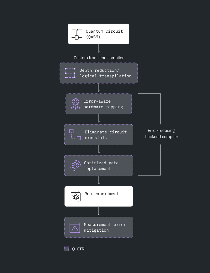
この関数は、「Sampler」と「Estimator」という 2 つのプリミティブを提供しており、両者の入力および出力は、 IBM Quantum V2 のプリミティブについて実装された仕様を拡張したものです。

ベンチマーク

公開されたアルゴリズムのベンチマーク結果では、Bernstein-Vazirani、量子フーリエ変換、Groverの探索、量子近似最適化アルゴリズム、変分量子固有値解法など、さまざまなアルゴリズムで大幅な性能向上が実証されています。このセクションの残りの部分では、実行可能なアルゴリズムの種類、予想されるパフォーマンスとランタイムの詳細を説明します。

以下の独立研究は、Q-CTRLのパフォーマンスマネジメントが、記録的な規模のアルゴリズム研究をいかに可能にしているかを実証しています：

ネットワークサービス障害診断のためのパラメトライズされたエネルギー効率に優れた量子カーネル - 最大50量子ビットの量子カーネル学習
大規模実証のためのテンソルベースの量子位相差推定 - 最大33量子ビットの量子位相推定
量子MLのための階層的学習：大規模変分量子回路のための新しい学習技法 - 21量子ビットの量子データロードまで

以下の表は、 ibm_fez で過去に実施されたベンチマークの精度と実行時間の大まかな目安です。他の機器での性能は異なる場合があります。使用時間は、1回線あたり10,000ショットを想定している。表示されている "量子ビット数 "は難しい制限ではなく、極めて安定した解の精度が期待できる大まかな閾値を表しています。より大きな問題サイズでも解決に成功しており、この限界を超えたテストが奨励されている。

例	量子ビット数	正確性	正確さの尺度	合計回数	ランタイム使用量 (s)	プリミティブ（モード）
バーンスタイン・バジラニ	50Q	100％	成功率（正解が最高カウントのビット列である実行の割合）	10	8	サンプラー
量子フーリエ変換	30Q	100％	成功率（正解が最高カウントのビット列である実行の割合）	10	8	サンプラー
量子位相推定	30Q	99.9998%	求めた角度の精度： `1- abs(real_angle - angle_found)/pi`	10	8	サンプラー
量子シミュレーションイジング模型（15ステップ）	20Q	99.775%	$A$ (以下に定義する）	60（1ステップあたり）	15（各ステップ）	推定法
量子シミュレーション2：分子動力学（20タイムポイント）	34Q	96.78%	$A_{mean}$ (以下に定義する）	10（各時点）	6（各時点）	推定法

期待値の測定精度の定義-指標 $A$ は以下のように定義される：

A = 1 - \frac{|\epsilon^{ideal} - \epsilon^{meas}|}{\epsilon^{ideal}_{max} - \epsilon^{ideal}_{min}},

ここで、 $\epsilon^{ideal}$ = 理想的な期待値、 $\epsilon^{meas}$ = 測定された期待値、 $\epsilon^{ideal}_{max}$ = 理想的な最大値、 $\epsilon^{ideal}_{min}$ = 理想的な最小値。 $A_{mean}$ は、単に複数の測定にわたる $A$ の値の平均である。

この指標が使われるのは、グローバルなシフトや到達可能な値の範囲でのスケーリングに対して不変だからだ。言い換えれば、期待値の可能性の範囲を上下にずらそうが、スプレッドを大きくしようが、 $A$ の値は一定であるべきなのだ。

使用を開始する

Fire Opal Performance Management では、推奨バージョン2.0.0である Qiskit v を使用しています。対応しているバージョンは、Qiskit v2.0.0.以上です。 IBM Quantum Platform のAPIキーを使用して認証を行い、次のようにQiskit Functionを選択してください。（このスニペットは、アカウントがすでにローカル環境に保存されていることを前提としています。）

from qiskit_ibm_catalog import QiskitFunctionsCatalog

catalog = QiskitFunctionsCatalog(channel="ibm_quantum_platform")

# verify that you have access to the function
catalog.list()

Output:

[QiskitFunction(qunova/hivqe-chemistry),
 QiskitFunction(global-data-quantum/quantum-portfolio-optimizer),
 QiskitFunction(algorithmiq/tem),
 QiskitFunction(qedma/qesem),
 QiskitFunction(multiverse/singularity),
 QiskitFunction(ibm/circuit-function),
 QiskitFunction(q-ctrl/optimization-solver),
 QiskitFunction(colibritd/quick-pde),
 QiskitFunction(q-ctrl/performance-management),
 QiskitFunction(kipu-quantum/iskay-quantum-optimizer)]

# Access Function
perf_mgmt = catalog.load("q-ctrl/performance-management")

この関数は、すべての IBM バックエンドに対応していますか？

この関数が現在サポートしていないバックエンドを使用したい場合は、 Q-CTRLまでご連絡いただき、サポートの追加をご依頼ください。

推定器プリミティブ

見積もりツールの例

Fire Opal Performance ManagementのEstimatorプリミティブを使用して、1つの回路と観測可能なペアの期待値を決定します。

qiskit-ibm-catalog 、 qiskit パッケージに加え、 numpy パッケージもこの例の実行に使用します。 IPythonカーネルを使ってこのサンプルをノートブックで実行している場合は、以下のセルをアンコメントすることでこのパッケージをインストールできます。

# %pip install numpy

1.回路を作る

例として、ランダムなエルミート演算子と観測値を生成し、パフォーマンス管理関数に入力する。

import numpy as np
from qiskit.circuit.library import iqp
from qiskit.quantum_info import random_hermitian, SparsePauliOp

n_qubits = 50

# Generate a random circuit
mat = np.real(random_hermitian(n_qubits, seed=1234))
circuit = iqp(mat)
circuit.measure_all()

# Define observables as a string
observable = SparsePauliOp("Z" * n_qubits)

# Create PUB tuple
estimator_pubs = [(circuit, observable)]

2.サーキットを走る

サーキットを走らせ、オプションでバックエンドとショット数を定義する。

# Run the circuit using Estimator
qctrl_estimator_job = perf_mgmt.run(
    primitive="estimator",
    pubs=estimator_pubs,
    backend_name=backend_name,
)

おなじみの Qiskit Serverless API を使用して、Qiskit Functionワークロードのステータスを確認できます：

qctrl_estimator_job.status()

Output:

'QUEUED'

3.結果の取得

# Retrieve the counts from the result list
result = qctrl_estimator_job.result()

結果は、Estimatorの結果と同じ形式になっています：

import numpy

result_str = str(result)

with numpy.printoptions(threshold=200):
    print(
        f"The result of the submitted job had {len(result)} PUB "
        f"and has a value:\n {result[0]}\n"
    )

print("The associated PubResult of this job has the following DataBins:")
print(f"{result[0].data}\n")

print(f"And this DataBin has attributes: {result[0].data.keys()}")

print("The expectation values measured from this PUB are:")
print(f"{result[0].data.evs}")

Output:

The result of the submitted job had 1 PUB
The result of the submitted job had 1 PUB and has a value:
 PubResult(data=DataBin(evs=0.0195, stds=0.9998098569228051), metadata={'precision': None})

The associated PubResult of this job has the following DataBins:
DataBin(evs=0.0195, stds=0.9998098569228051)

And this DataBin has attributes: dict_keys(['evs', 'stds'])
The expectation values measured from this PUB are:
0.0195

サンプラープリミティブ

サンプラーの例

Fire Opal Performance ManagementのSamplerプリミティブを使用して、Bernstein-Vazirani回路を実行します。ブラックボックス関数の出力から隠れた文字列を見つけるために使われるこのアルゴリズムは、正解が1つであるため、一般的なベンチマークアルゴリズムである。

1.回路を作る

アルゴリズム、隠しビット列、Bernstein-Vazirani 回路の正解を定義しなさい。 circuit_width を変えるだけで、回路の幅を調整できる。

import qiskit

circuit_width = 35
hidden_bitstring = "1" * circuit_width

# Create circuit, reserving one qubit for BV oracle
bv_circuit = qiskit.QuantumCircuit(circuit_width + 1, circuit_width)
bv_circuit.x(circuit_width)
bv_circuit.h(range(circuit_width + 1))
for input_qubit, bit in enumerate(reversed(hidden_bitstring)):
    if bit == "1":
        bv_circuit.cx(input_qubit, circuit_width)
bv_circuit.barrier()
bv_circuit.h(range(circuit_width + 1))
bv_circuit.barrier()
for input_qubit in range(circuit_width):
    bv_circuit.measure(input_qubit, input_qubit)

# Create PUB tuple
sampler_pubs = [(bv_circuit,)]

2.サーキットを走る

サーキットを走らせ、オプションでバックエンドとショット数を定義する。

# Run the circuit using Sampler
qctrl_sampler_job = perf_mgmt.run(
    primitive="sampler",
    pubs=sampler_pubs,
    backend_name=backend_name,
)

Qiskit Function ワークロードのステータスを確認したり、結果を返したりするには、次のように操作してください：

# Print the ID so you can use it later, if necessary
print(qctrl_sampler_job.job_id)

qctrl_sampler_job.status()

Output:

60fe2fa1-a860-43e4-8615-c6ac4180f93b

'QUEUED'

3.結果の取得

# Retrieve the job results
sampler_result = qctrl_sampler_job.result()

# Get results for the first (and only) PUB
pub_result = sampler_result[0]
counts = pub_result.data.c.get_counts()

print("Counts for the meas output register (limited to 30 results):")
for i, (bitstring, count) in enumerate(counts.items()):
    if i >= 50:
        print(f"  ... ({len(counts) - 30} more items)")
        break
    print(f"  {bitstring}: {count}")

Output:

Counts for the meas output register (limited to 30 results):
  11111111111111111111111111111111111: 1661
  11111111111111111111111111110111111: 60
  11111111111111111111111111111101111: 54
  11111111111111111111111111111110111: 54
  11111111111111011111111111111111111: 46
  11111111111111111110111111111111111: 44
  11111111111111111111111101111111111: 42
  11111111111111111111111110111111111: 42
  11111111111111110111111111111111111: 41
  11111111111111111111111111111111101: 39
  11111111111111111111101111111111111: 38
  11111111111111111111110111111111111: 38
  11111111111111111111111111101111111: 37
  11111111111111111111111111111111110: 36
  11111111111110111111111111111111111: 35
  11111111111111111111111111111011111: 32
  11111111111111101111111111111111111: 32
  01111111111111111111111111111111111: 27
  11111111111111111011111111111111111: 23
  11111111101111111111111111111111111: 22
  11111111111111111111111111111111011: 21
  11111111011111111111111111111111111: 20
  00000000000000011111111111111111111: 18
  11111111111111111111110101111111111: 18
  00000001111111111111111111111111111: 17
  11111111001111111111111111111111111: 16
  11101111111111111111111111111111111: 16
  11111111111101111111111111111111111: 16
  00000101111111111111111111111111111: 13
  11111111111111111111111011111111111: 13
  11111111111111111111111110101111111: 13
  11111111111111111101111111111111111: 12
  10111111111111111111111111111111111: 12
  11111111111111111111111110001111111: 12
  00000000000000000011111111111111111: 11
  11111111111111111111111111111110110: 10
  00000000000000000000000001111111111: 10
  11111111111011111111111111111111111: 9
  11111111111111101011111111111111111: 9
  00000000011111111111111111111111111: 8
  10101111111111111111111111111111111: 8
  00000000000000000000000001011111111: 8
  11111111111111111111111111111111001: 8
  00000111111111111111111111111111111: 7
  11111111111111111111111111111101110: 7
  11111111110111111111111111111111111: 7
  00000000000001011111111111111111111: 6
  00000000000000001111111111111111111: 6
  00000000000000000001011111111111111: 6
  11111111111111111111111111011111111: 6
  ... (1050 more items)

3.上位のビット列をプロットする

隠されたビット列がモードであったかどうかを確認するために、カウント数の最も多いビット列をプロットする。

import matplotlib.pyplot as plt


def plot_top_bitstrings(counts_dict, hidden_bitstring=None):
    # Sort and take the top 100 bitstrings
    top_100 = sorted(counts_dict.items(), key=lambda x: x[1], reverse=True)[
        :100
    ]
    if not top_100:
        print("No bitstrings found in the input dictionary.")
        return

    # Unzip the bitstrings and their counts
    bitstrings, counts = zip(*top_100)

    # Assign colors: purple if the bitstring matches hidden_bitstring,
    # otherwise gray
    colors = [
        "#680CE9" if bit == hidden_bitstring else "gray" for bit in bitstrings
    ]

    # Create the bar plot
    plt.figure(figsize=(15, 8))
    plt.bar(
        range(len(bitstrings)), counts, tick_label=bitstrings, color=colors
    )

    # Rotate the bitstrings for better readability
    plt.xticks(rotation=90, fontsize=8)
    plt.xlabel("Bitstrings")
    plt.ylabel("Counts")
    plt.title("Top 100 Bitstrings by Counts")

    # Show the plot
    plt.tight_layout()
    plt.show()

隠されたビット列は紫色で強調表示され、カウント数が最も多いビット列でなければならない。

plot_top_bitstrings(counts, hidden_bitstring)

Output:

変更ログ

2026-02-20: 非推奨通知 - メタデータフィールド provider_job_ids は、バージョン 0.13.0 において30日後に非推奨となります。ユーザーはランタイムサービスのメソッド job_id() を通じてジョブIDにアクセスできます。
2026-02-11: 現在はのサポートを提供 ibm_miamiし、に実行メタ PubResultデータを追加しました。

サポートの利用

ご質問や問題がございましたら、 Q-CTRLまでお問い合わせください。

次のステップ

推奨事項

Q-CTRL パフォーマンス管理へのアクセス権を申請してください。
このQiskit関数の APIリファレンスをご覧ください。
Q-CTRLのパフォーマンス管理チュートリアルで横磁場イジングモデルを試してみてください。
Q-CTRLの Qiskit Functions チュートリアルで量子位相推定を試す
レビューマンダダ P. S et al. (2023). 量子アルゴリズム向け自動化された決定論的エラー抑制ワークフローの実験的ベンチマーク評価 Physical Review Applied, 20, 2.
レビュー菅野, S., et al. (2025). 大規模実証のためのテンソルベース量子位相差推定 arXiv プレプリント arXiv:2408.04946.
レビュー： SoftBank 社、量子 Machine Learning を用いた通信サービス障害診断システムのデモンストレーション実験（ブログ）、2024年8月30日。
レビュー山内英樹, et al. (2024). ネットワークサービス障害診断のためのパラメータ化エネルギー効率型量子カーネル arXiv プレプリント arXiv:2405.09724v1.
レビュー山内英樹, et al. (2025). 超対称ハミルトニアンによるトポロジカルダイナミクスの量子分光法 arXiv プレプリント arXiv:2511.23169v1.
王、Y. のレビュー et al. (2025). Δ-モチーフ：データ中心並列処理による大規模サブグラフ同型性問題 arXiv プレプリント arXiv:2508.21287.
レビューパテラキス, N. G., et al. (2025). パワーエレクトロニクスの計算環境における量子コンピューティング：展望と現状 arXiv プレプリント arXiv:2507.02577.
レビューガリビアン, H., et al. (2023). 量子機械学習のための階層的学習：大規模変分量子回路のための新規トレーニング手法 arXiv プレプリント arXiv:2311.12929.
三菱化学株式会社のケーススタディを検討する。
編集済み銀行ケーススタディを確認する。
BlueQubit のケーススタディを確認する。

このページは役に立ちましたか？

バグや誤字の報告、またはコンテンツの要求はGitHubで行ってください。